Type-Driven Development with Idris
Edwin Brady
![]()
Copyright
For online information and ordering of this and other Manning books, please visit www.manning.com. The publisher offers discounts on this book when ordered in quantity. For more information, please contact
Special Sales Department Manning Publications Co. 20 Baldwin Road PO Box 761 Shelter Island, NY 11964 Email: orders@manning.com
©2017 by Manning Publications Co. All rights reserved.
No part of this publication may be reproduced, stored in a retrieval system, or transmitted, in any form or by means electronic, mechanical, photocopying, or otherwise, without prior written permission of the publisher.
Many of the designations used by manufacturers and sellers to distinguish their products are claimed as trademarks. Where those designations appear in the book, and Manning Publications was aware of a trademark claim, the designations have been printed in initial caps or all caps.
 Recognizing the importance of preserving what has been written, it is Manning’s policy to have the books we publish printed on acid-free paper, and we exert our best efforts to that end. Recognizing also our responsibility to conserve the resources of our planet, Manning books are printed on paper that is at least 15 percent recycled and processed without the use of elemental chlorine.
 | Manning Publications Co. 20 Baldwin Road PO Box 761 Shelter Island, NY 11964 |
Development editor: Dan Maharry Review editor: Aleksandar Dragosavljević Technical development editor: Andrew Gibson Project editor: Kevin Sullivan Copyeditor: Andy Carroll Proofreader: Katie Tennant Technical proofreaders: Arnaud Bailly, Nicolas Biri Typesetter: Dottie Marsico Cover designer: Marija Tudor
ISBN 9781617293023
Printed in the United States of America
1 2 3 4 5 6 7 8 9 10 – EBM – 22 21 20 19 18 17
Brief Table of Contents
Chapter 3. Interactive development with types
Chapter 4. User-defined data types
Chapter 5. Interactive programs: input and output processing
Chapter 6. Programming with first-class types
Chapter 7. Interfaces: using constrained generic types
Chapter 8. Equality: expressing relationships between data
Chapter 9. Predicates: expressing assumptions and contracts in types
Chapter 11. Streams and processes: working with infinite data
Chapter 12. Writing programs with state
Chapter 13. State machines: verifying protocols in types
Chapter 14. Dependent state machines: handling feedback and errors
Appendix A. Installing Idris and editor modes
Table of Contents
1.2. Introducing type-driven development
1.2.2. An automated teller machine
1.2.4. Type, define, refine: the process of type-driven development
1.3. Pure functional programming
1.3.1. Purity and referential transparency
1.4.1. The interactive environment
1.4.3. Compiling and running Idris programs
Chapter 2. Getting started with Idris
2.1.1. Numeric types and values
2.2. Functions: the building blocks of Idris programs
2.2.1. Function types and definitions
2.2.2. Partially applying functions
2.2.3. Writing generic functions: variables in types
2.2.4. Writing generic functions with constrained types
Chapter 3. Interactive development with types
3.1. Interactive editing in Atom
3.1.1. Interactive command summary
3.2. Adding precision to types: working with vectors
3.2.1. Refining the type of allLengths
3.3. Example: type-driven development of matrix functions
3.4. Implicit arguments: type-level variables
3.4.1. The need for implicit arguments
Chapter 4. User-defined data types
4.2. Defining dependent data types
4.2.1. A first example: classifying vehicles by power source
4.3. Type-driven implementation of an interactive data store
4.3.2. Interactively maintaining state in main
Chapter 5. Interactive programs: input and output processing
5.1. Interactive programming with IO
5.1.1. Evaluating and executing interactive programs
5.2. Interactive programs and control flow
5.2.1. Producing pure values in interactive definitions
5.3. Reading and validating dependent types
5.3.1. Reading a Vect from the console
Chapter 6. Programming with first-class types
6.1. Type-level functions: calculating types
6.1.1. Type synonyms: giving informative names to complex types
6.2. Defining functions with variable numbers of arguments
6.3. Enhancing the interactive data store with schemas
6.3.1. Refining the DataStore type
6.3.2. Using a record for the DataStore
6.3.3. Correcting compilation errors using holes
6.3.4. Displaying entries in the store
Chapter 7. Interfaces: using constrained generic types
7.1. Generic comparisons with Eq and Ord
7.1.1. Testing for equality with Eq
7.1.2. Defining the Eq constraint using interfaces and implementations
7.1.3. Default method definitions
7.2. Interfaces defined in the Prelude
7.3. Interfaces parameterized by Type -> Type
7.3.1. Applying a function across a structure with Functor
Chapter 8. Equality: expressing relationships between data
8.1. Guaranteeing equivalence of data with equality types
8.1.1. Implementing exactLength, first attempt
8.1.2. Expressing equality of Nats as a type
8.1.3. Testing for equality of Nats
8.1.4. Functions as proofs: manipulating equalities
8.2. Equality in practice: types and reasoning
8.2.2. Type checking and evaluation
8.2.3. The rewrite construct: rewriting a type using equality
8.3. The empty type and decidability
8.3.1. Void: a type with no values
Chapter 9. Predicates: expressing assumptions and contracts in types
9.1. Membership tests: the Elem predicate
9.1.1. Removing an element from a Vect
9.1.2. The Elem type: guaranteeing a value is in a vector
9.1.3. Removing an element from a Vect: types as contracts
9.1.4. auto-implicit arguments: automatically constructing proofs
9.1.5. Decidable predicates: deciding membership of a vector
9.2. Expressing program state in types: a guessing game
9.2.1. Representing the game’s state
9.2.2. A top-level game function
9.2.3. A predicate for validating user input: ValidInput
Chapter 10. Views: extending pattern matching
10.1. Defining and using views
10.1.1. Matching the last item in a list
10.1.2. Building views: covering functions
10.1.3. with blocks: syntax for extended pattern matching
10.2. Recursive views: termination and efficiency
10.2.1. “Snoc” lists: traversing a list in reverse
10.2.2. Recursive views and the with construct
10.3. Data abstraction: hiding the structure of data using views
10.3.1. Digression: modules in Idris
Chapter 11. Streams and processes: working with infinite data
11.1. Streams: generating and processing infinite lists
11.1.1. Labeling elements in a List
11.1.2. Producing an infinite list of numbers
11.1.3. Digression: what does it mean for a function to be total?
11.2. Infinite processes: writing interactive total programs
11.2.1. Describing infinite processes
11.2.2. Executing infinite processes
11.2.3. Executing infinite processes as total functions
11.2.4. Generating infinite structures using Lazy types
11.3. Interactive programs with termination
11.3.1. Refining InfIO: introducing termination
Chapter 12. Writing programs with state
12.1. Working with mutable state
12.1.1. The tree-traversal example
12.1.2. Representing mutable state using a pair
12.2. A custom implementation of State
12.2.1. Defining State and runState
12.2.2. Defining Functor, Applicative, and Monad implementations for State
12.3. A complete program with state: working with records
12.3.1. Interactive programs with state: the arithmetic quiz revisited
12.3.2. Complex state: defining nested records
12.3.3. Updating record field values
12.3.4. Updating record fields by applying functions
12.3.6. Running interactive and stateful programs: executing the quiz
Chapter 13. State machines: verifying protocols in types
13.1. State machines: tracking state in types
13.1.1. Finite state machines: modeling a door as a type
13.1.2. Interactive development of sequences of door operations
13.2. Dependent types in state: implementing a stack
13.2.1. Representing stack operations in a state machine
13.2.2. Implementing the stack using Vect
13.2.3. Using a stack interactively: a stack-based calculator
Chapter 14. Dependent state machines: handling feedback and errors
14.1. Dealing with errors in state transitions
14.1.1. Refining the door model: representing failure
14.1.2. A verified, error-checking, door-protocol description
14.2. Security properties in types: modeling an ATM
14.2.1. Defining states for the ATM
14.2.2. Defining a type for the ATM
14.3. A verified guessing game: describing rules in types
14.3.1. Defining an abstract game state and operations
14.3.2. Defining a type for the game state
Chapter 15. Type-safe concurrent programming
15.1. Primitives for concurrent programming in Idris
15.1.1. Defining concurrent processes
15.2. Defining a type for safe message passing
15.2.1. Describing message-passing processes in a type
15.2.2. Making processes total using Inf
15.2.3. Guaranteeing responses using a state machine and Inf
15.2.4. Generic message-passing processes
15.2.5. Defining a module for Process
Appendix A. Installing Idris and editor modes
The Idris compiler and environment
Appendix B. Interactive editing commands
Functional programming in Haskell
Preface
Computers are everywhere, and we rely on software daily. As well as running our desktop and laptop computers, software controls our communications, banking, transport infrastructure, and even our domestic appliances. Even so, it’s considered a fact of life that software is unreliable. If a laptop or mobile phone fails, it’s merely inconvenient and requires a restart (possibly accompanied by cursing over losing the last few minutes of work). If, on the other hand, the software controlling a business-critical application or server fails, significant time and money can be lost. For safety-critical systems, the repercussions could be even worse.
For many years, therefore, computer science researchers have been searching for ways to improve the robustness and safety of software. One approach among many is to use types to describe what a program is supposed to do. In particular, by using dependent types, you describe precise properties of a program. The idea is that if you can express a program’s intention in its type, and the program successfully type-checks, then the program must behave as intended. An important (if ambitious and long-term) goal of the Idris programming language is to make the results of this research accessible to software developers in general, and correspondingly reduce the possibility of critical software failures.
Initially, this book’s focus was programming in Idris: showing how to use its type system to guarantee important properties of programs. Under the guidance of development editor Dan Maharry, and thanks to the efforts of technical development editor Andrew Gibson, it has evolved to become as much about the process of programming with dependent types as about how the resulting programs work. You’ll learn about the fundamentals of dependent types, how to use types to define programs interactively, and how to refine programs and types as your understanding of a problem evolves. You’ll also learn about some real-world applications of type-driven development, particularly in dealing with state, protocols, and concurrency.
Idris itself arose as a result of my own research into program verification and language design with dependent types. After spending several years immersed in the concept of programming with dependent types, I felt there was a need for a language designed for developers as well as researchers. I hope that you have as much fun learning about type-driven development with Idris as I have had developing it!
Acknowledgments
Many people have helped in the writing of this book, and it wouldn’t exist without them. In particular, I thank Dan Maharry, who encouraged me to reveal the ideas of type-driven development much more clearly. The mantra of “type, define, refine,” which appears throughout the book, was Dan’s suggestion. I also owe many thanks to Andrew Gibson, who has meticulously worked through all the examples and exercises throughout the book, making sure they work, checking that the exercises are solvable, and suggesting many improvements to the text and explanations. Overall, I’d like to thank the team at Manning Publications for helping to make this book a reality.
The design of Idris owes much to several decades of research into type theory, functional programming, and language design. I’m grateful to James McKinna and Conor McBride in particular for teaching me the fundamentals of type theory when I was a graduate student at Durham University, and for their continued advice and encouragement since. I’d also like to thank the researchers and developers responsible for the languages and systems that have inspired my work, namely, tools such as Haskell, Epigram, Agda, and Coq. Idris couldn’t exist without the work that has come before, and I can only hope that it, in turn, inspires others in the future. See appendix D for some references to the work that inspired Idris.
Several colleagues and students at the University of St. Andrews and elsewhere have provided useful feedback on earlier drafts of chapters and have been patient while I worked on the book instead of working on other things. In particular, I would like to thank Ozgur Akgun, Nicola Botta, Sam Elliot, Simon Fowler, Nicolas Gagliani (who contributed the extension to the Atom editor that you’ll use throughout the book), Jan de Muijnck-Hughes, Markus Pfeiffer, Chris Schwaab, and Matúš Tejiščák for their comments and suggestions. My sincere apologies to anyone else I’ve forgotten to name!
Readers who have purchased early access and reviewers of earlier drafts have contributed many useful comments and suggestions. Those reviewers include Alexander A. Myltsev, Álvaro Falquina, Arnaud Bailly, Carsten Jørgensen, Christine Koppelt, Giovanni Ruggiero, Ian Dees, Juan Gabriel Bono, Mattias Lundell, Phil de Joux, Rintcius Blok, Satadru Roy, Sergey Selyugin, Todd Fine, and Vitaly Bragilevsky.
I couldn’t have implemented Idris on my own. Since I began developing the current version in late 2011, there have been many contributors, but most of all I would like to thank David Christiansen, who is responsible for much of the polish in the Idris REPL and the interactive editing tools; he has also worked hard to help newcomers to the project. Thanks are also due to the other contributors: Ozgur Akgun, Ahmad Salim Al-Sibahi, Edward Chadwick Amsden, Michael R. Bernstein, Jan Bessai, Nicola Botta, Vitaly Bragilevsky, Jakob Brünker, Alyssa Carter, Carter Charbonneau, Aaron Craelius, Jason Dagit, Adam Sandberg Eriksson, Guglielmo Fachini, Simon Fowler, Zack Grannan, Sean Hunt, Cezar Ionescu, Heath Johns, Irene Knapp, Paul Koerbitz, Niklas Larsson, Shea Levy, Mathnerd314, Hannes Mehnert, Mekeor Melire, Melissa Mozifian, Jan de Muijnck-Hughes, Dominic Mulligan, Echo Nolan, Tom Prince, raichoo, Philip Rasmussen, Aistis Raulinaitis, Reynir Reynisson, Seo Sanghyeon, Benjamin Saunders, Alexander Shabalin, Jeremy W. Sherman, Timo Petteri Sinnemäki, JP Smith, startling, Chetan T, Matúš Tejiščák, Dirk Ullrich, Leif Warner, Daniel Waterworth, Eric Weinstein, Jonas Westerlund, Björn Aili, and Zheng Jihui.
Finally, thanks go to my parents, whose purchase of a BBC Micro in 1983 set me off on this path; and to Emma, for waiting so patiently for me to finish this, and for bringing me coffee to keep me going.
About this Book
Type-Driven Development with Idris is about making types work for you. Types are often seen as a tool for checking for errors, with the programmer writing a complete program first and using the type checker to detect errors. In type-driven development, you use types as a tool for constructing programs, and the type checker as your assistant to guide you to a complete and working program.
This book begins by describing what you can express with types; then, it introduces the core features of the Idris programming language. Finally, it describes some more-practical applications of type-driven development.
Who should read this book
This book is aimed at developers who want to learn about the state of the art in using sophisticated type systems to help develop robust software. It aims to provide an accessible introduction to dependent types, and to show how modern type-based techniques can be applied to real-world problems.
Readers will ideally already be familiar with functional programming concepts such as closures and higher-order functions, although the book introduces these and other concepts as necessary. Knowledge of another functional programming language such as Haskell, OCaml, or Scala will be particularly helpful, though none is assumed.
Roadmap
This book is divided into three parts. Part 1 (chapters 1 and 2) introduces the concepts and gives a tour of the Idris programming language:
- Chapter 1 introduces type-driven development and gets you started with the Idris environment.
- Chapter 2 covers the basics of Idris programming, including primitive types and structuring Idris programs.
Part 2 (chapters 3–10) introduces the core language features of Idris:
- Chapter 3 discusses interactive development using the Atom editor and describes how using more-precise types means that the type checker can help you write programs.
- Chapter 4 explains how to define your own data types and presents a first example of writing a larger interactive program in the type-driven style.
- Chapter 5 describes interactive programs in more depth, including how to use types to help validate user inputs to interactive programs.
- Chapter 6 introduces type-level programming, showing how to write functions that calculate types and how to use them in practice.
- Chapter 7 describes how to use interfaces to write programs with generic types.
- Chapter 8 explains how you can use types to express relationships between data, particularly to describe properties of data and to guarantee that functions behave a certain way.
- Chapter 9 explains further how types can express contracts that functions must satisfy, including an example that shows how to use types to describe the state of a system.
- Chapter 10 introduces views, which are alternative ways of inspecting and traversing data structures.
Part 3 (chapters 11–15) describes some applications of Idris to real-world software development, particularly working with state and interactive programs:
- Chapter 11 describes how to work with potentially infinite data, such as streams, and how to write and reason about interactive programs that could run indefinitely.
- Chapter 12 explains how to write programs with state and how to represent and manipulate complex state using records.
- Chapter 13 shows how to express a state machine in an Idris type, and how to use the type to guarantee that programs follow protocols correctly.
- Chapter 14 describes more-sophisticated state machines, how to handle errors and feedback from an environment, and how to represent security properties of a system in its type.
- Chapter 15 concludes the book with a worked example: type-driven development of a small library for concurrent programming.
In general, each chapter builds on concepts introduced in earlier chapters, so it’s intended that you read the chapters in order. Most importantly, the book describes the process of type-driven development and constructing programs interactively from a type. Therefore, I strongly recommend working through the examples on a computer as you read. Furthermore, if you’re reading the eBook, type in the examples—don’t just copy and paste.
There are exercises throughout each chapter, so, as you read, make sure that you complete the exercises to reinforce your understanding. Sample solutions are available online from the book’s website at www.manning.com/books/type-driven-development-with-idris.
There are four appendices: Appendix A describes how to install Idris and the Atom editor mode, which we’ll use throughout the book. Appendix B summarizes the interactive editing commands supported by Atom. Appendix C summarizes the commands you can use in the Idris environment. Finally, appendix D gives references to some of the work that inspired Idris, and where you can learn more about the theoretical background and related tools.
Code conventions and downloads
This book contains many examples of source code both in numbered listings and inline with normal text. In both cases, source code is formatted in a fixed-width font like this to separate it from ordinary text.
In many cases, the original source code has been reformatted; I’ve added line breaks and reworked indentation to accommodate the available page space in the book. Additionally, comments in the source code have often been removed from the listings when the code is described in the text. Code annotations accompany many of the listings, highlighting important concepts.
All of the code in this book is available online from the book’s website (www.manning.com/books/type-driven-development-with-idris) and has been tested with Idris 1.0. The code is also available in a Git repository here: https://github.com/edwinb/TypeDD-Samples.
Author Online
Purchase of Type-Driven Development with Idris includes free access to a private web forum run by Manning Publications where you can make comments about the book, ask technical questions, and receive help from the author and from other users. To access the forum and subscribe to it, point your web browser to www.manning.com/books/type-driven-development-with-idris. This page provides information on how to get on the forum once you’re registered, what kind of help is available, and the rules of conduct on the forum.
Manning’s commitment to our readers is to provide a venue where a meaningful dialog between individual readers and between readers and the author can take place. It’s not a commitment to any specific amount of participation on the part of the author, whose contribution to the forum remains voluntary (and unpaid). We suggest you try asking him challenging questions lest his interest stray!
The Author Online forum and the archives of previous discussions will be accessible from the publisher’s website as long as the book is in print.
Other online resources
If you’d like to learn more about Idris, you can find more resources on the Idris website: http://idris-lang.org/. You can also find help in several other places:
- The idris-lang Google Group is an active group discussing all aspects of Idris. The group welcomes questions from beginners and more-advanced users alike.
- There is an IRC channel, #idris on irc.freenode.net, which is similarly open to questions.
- You can ask and answer questions using the Idris tag on Stack Overflow.
About the Author

EDWIN BRADY leads the design and implementation of the Idris programming language. He is a lecturer in Computer Science at the University of St. Andrews in Scotland, and he regularly speaks at conferences. When he’s not doing that, you might find him playing a game of Go, watching a game of cricket, or somewhere up a hill in the middle of Scotland.
About the Cover Illustration
The figure on the cover of Type-Driven Development with Idris is captioned “La Gasconne,” or “A woman from Gascony.” The illustration is taken from a collection of works by many artists, edited by Louis Curmer and published in Paris in 1841. The title of the collection is Les Français peints par eux-mêmes, which translates as The French People Painted by Themselves. Each illustration is finely drawn and colored by hand, and the rich variety of drawings in the collection reminds us vividly of how culturally apart the world’s regions, towns, villages, and neighborhoods were just 200 years ago. Isolated from each other, people spoke different dialects and languages. In the streets or in the countryside, it was easy to identify where they lived and what their trade or station in life was just by their dress.
Dress codes have changed since then, and the diversity by region, so rich at the time, has faded away. It’s now hard to tell apart the inhabitants of different continents, let alone different towns or regions. Perhaps we have traded cultural diversity for a more varied personal life—certainly for a more varied and fast-paced technological life.
At a time when it’s hard to tell one computer book from another, Manning celebrates the inventiveness and initiative of the computer business with book covers based on the rich diversity of regional life of two centuries ago, brought back to life by pictures from collections such as this one.
Part 1. Introduction
In this first part, you’ll get started with Idris and learn about the ideas behind type-driven development. I’ll take you on a brief tour of the Idris environment, and you’ll write some simple but complete programs.
In the first chapter, I’ll explain more about what I mean by type-driven development. Most importantly, I’ll define what I mean by “type” and give several examples of how you can use expressive types to describe the intended purpose of your programs more precisely. I’ll also introduce the two most distinctive features of the Idris language: holes, which stand for parts of programs that are yet to be written, and the use of types as a first-class language construct.
Before you get too deeply into type-driven development in Idris, it’s important to have a solid grasp of the fundamentals of the language. Therefore, in chapter 2, I’ll discuss some of the primitive language constructs, many of which will be familiar to you from other languages, and show how to construct complete programs in Idris.
Chapter 1. Overview
This chapter covers
- Introducing type-driven development
- The essence of pure functional programming
- First steps with Idris
This book teaches a new approach to building robust software, type-driven development, using the Idris programming language. Traditionally, types are seen as a tool for checking for errors, with the programmer writing a complete program first and using either the compiler or the runtime system to detect type errors. In type-driven development, we use types as a tool for constructing programs. We put the type first, treating it as a plan for a program, and use the compiler and type checker as our assistant, guiding us to a complete and working program that satisfies the type. The more expressive the type is that we give up front, the more confidence we can have that the resulting program will be correct.
Types and tests
The name “type-driven development” suggests an analogy to test-driven development. There’s a similarity, in that writing tests first helps establish a program’s purpose and whether it satisfies some basic requirements. The difference is that, unlike tests, which can usually only be used to show the presence of errors, types (used appropriately) can show the absence of errors. But although types reduce the need for tests, they rarely eliminate it entirely.
In Idris, types are a first-class language construct. Types can be manipulated, used, passed as arguments to functions, and returned from functions just like any other value, such as numbers, strings, or lists. This is a simple but powerful idea:
- It allows relationships to be expressed between values; for example, that two lists have the same length.
- It allows assumptions to be made explicit and checkable by the compiler. For example, if you assume that a list is non-empty, Idris can ensure this assumption always holds before the program is run.
- If desired, it allows program behavior to be formally stated and proven correct.
In this chapter, I’ll introduce the Idris programming language and give a brief tour of its features and environment. I’ll also provide an overview of type-driven development, discussing why types matter in programming languages and how they can be used to guide software development. But first, it’s important to understand exactly what we mean when we talk about “types.”
1.1. What is a type?
We’re taught from an early age to recognize and distinguish types of objects. As a young child, you may have had a shape-sorter toy. This consists of a box with variously shaped holes in the top (see figure 1.1) and some shapes that fit through the holes. Sometimes they’re equipped with a small plastic hammer. The idea is to fit each shape (think of this as a “value”) into the appropriate hole (think of this as a “type”), possibly with coercion from the hammer.
Figure 1.1. The top of a shape-sorter toy. The shapes correspond to the types of objects that will fit through the holes.
In programming, types are a means of classifying values. For example, the values 94, "thing", and [1,2,3,4,5] could respectively be classified as an integer, a string, and a list of integers. Just as you can’t put a square shape in a round hole in the shape sorter, you can’t use a string like "thing" in a part of a program where you need an integer.
All modern programming languages classify values by type, although they differ enormously in when and how they do so (for example, whether they’re checked statically at compile time or dynamically at runtime, whether conversions between types are automatic or not, and so on).
Types serve several important roles:- For a machine, types describe how bit patterns in memory are to be interpreted.
- For a compiler or interpreter, types help ensure that bit patterns are interpreted consistently when a program runs.
- For a programmer, types help name and organize concepts, aiding documentation and supporting interactive editing environments.
From our point of view in this book, the most important purpose of types is the third. Types help programmers in several ways:
- By allowing for the naming and organization of concepts (such as Square, Circle, Triangle, and Hexagon)
- By providing explicit documentation of the purposes of variables, functions, and programs
- By driving code completion in an interactive editing environment
As you’ll see, type-driven development makes extensive use of code completion in particular. Although all modern, statically typed languages support code completion to some extent, the expressivity of the Idris type system leads to powerful automatic code generation.
1.2. Introducing type-driven development
Type-driven development is a style of programming in which we write types first and use those types to guide the definition of functions. The overall process is to write the necessary data types, and then, for each function, do the following:
- Write the input and output types.
- Define the function, using the structure of the input types to guide the implementation.
- Refine and edit the type and function definition as necessary.
When you write a program, you’ll often have a conceptual model in your head (or, if you’re disciplined, even on paper) of how it’s supposed to work, how the components interact, and how the data is organized. This model is likely to be quite vague at first and will become more precise as the program evolves and your understanding of the concept develops.
Types allow you to make these models explicit in code and ensure that your implementation of a program matches the model in your head. Idris has an expressive type system that allows you to describe a model as precisely as you need, and to refine the model at the same time as developing the implementation.
In type-driven development, instead of thinking of types in terms of checking, with the type checker criticizing you when you make a mistake, you can think of types as being a plan, with the type checker acting as your guide, leading you to a working, robust program. Starting with a type and an empty function body, you gradually add details to the definition until it’s complete, regularly using the
compiler to check that the program so far satisfies the type. Idris, as you’ll soon see, strongly encourages this style of programming by allowing incomplete function definitions to be checked, and by providing an expressive language for describing types.To illustrate further, in this section I’ll show some examples of how you can use types to describe in detail what a program is intended to do: matrix arithmetic, modeling an automated teller machine (ATM), and writing concurrent programs. Then, I’ll summarize the process of type-driven development and introduce the concept of dependent types, which will allow you to express detailed properties of your programs.
1.2.1. Matrix arithmetic
A matrix is a rectangular grid of numbers, arranged in rows and columns. They have several scientific applications, and in programming they have applications in cryptography, 3D graphics, machine learning, and data analytics. The following, for example, is a 3 × 4 matrix:
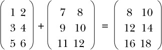
You can implement various arithmetic operations on matrices, such as addition and multiplication. To add two matrices, you add the corresponding elements, as you see here:
When programming with matrices, if you begin by defining a Matrix data type, then addition requires two inputs of type Matrix and gives an output of type Matrix. But because adding matrices involves adding corresponding elements of the inputs, what happens if the two inputs have different dimensions, as here?
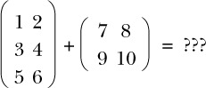
It’s likely that if you’re trying to add matrices of different dimensions, then you’ve made a mistake somewhere. So, instead of using a Matrix type, you could refine the
type so that it includes the dimensions of the matrix, and require that the two input matrices have the same dimensions:- The first example of a 3 × 4 matrix now has type Matrix 3 4.
- The first (correct) example of addition takes two inputs of type Matrix 3 2 and gives an output of type Matrix 3 2.
By including the dimensions in the type of a matrix, you can describe the input and output types of addition in such a way that it’s a type error to try to add matrices of different sizes. If you try to add a Matrix 3 2 and a Matrix 2 2, your program won’t compile, let alone run.
If you include the dimensions of a matrix in its type, then you need to think about the relationship between the dimensions of the input and output for every matrix operation. For example, transposing a matrix involves switching the rows to columns and vice versa, so if you transpose a 3 × 2 matrix, you’ll end up with a 2 × 3 matrix:
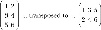
The input type of this transposition is Matrix 3 2, and the output type is Matrix 2 3.
In general, rather than giving exact dimensions in the type, we’ll use variables to describe the relationship between the dimensions of the inputs and the dimensions of the outputs. Table 1.1 shows the relationships between the dimensions of inputs and outputs for three matrix operations: addition, multiplication, and transposition.
Table 1.1. Input and output types for matrix operations. The names x, y, and z describe, in general, how the dimensions of the inputs and outputs are related.
| Operation | Input types | Output type |
|---|---|---|
| Add | Matrix x y, Matrix x y | Matrix x y |
| Multiply | Matrix x y, Matrix y z | Matrix x z |
| Transpose | Matrix x y | Matrix y x |
We’ll look at matrices in depth in chapter 3, where we’ll work through an implementation of matrix transposition in detail.
1.2.2. An automated teller machine
As well as using types to describe the relationships between the inputs and outputs of functions, as with matrix operations, you can describe precisely when operations are valid. For example, if you’re implementing software to drive an ATM, you’ll want to guarantee that the machine will dispense cash only after a user has entered a card and validated their personal identification number (PIN).
To see how this works, we’ll need to consider the possible states that an ATM can be in:
- Ready—The ATM is ready and waiting for a user to insert a card.
- CardInserted—The ATM is waiting for a user, having inserted a card, to enter their PIN.
- Session—A validated session is in progress, with the ATM, having validated the user’s PIN, ready to dispense cash.
An ATM supports several basic operations, each of which is valid only when the machine is in a specific state, and each of which might change the state of the machine, as illustrated in figure 1.2. These are the basic operations:
- InsertCard—Waits for the user to insert a card
- EjectCard—Ejects a card from the machine
- GetPIN—Prompts the user to enter a PIN
- CheckPIN—Checks whether an entered PIN is correct
- Dispense—Dispenses cash
Figure 1.2. The states and valid operations on an ATM. Each operation is valid only in specific states and can change the state of the machine. CheckPIN changes the state only if the entered PIN is correct.
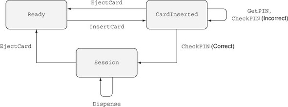
Whether an operation is valid or not depends on the state of the machine. For example, InsertCard is valid only in the Ready state, because that’s the only state where there’s no card already in the machine. Also, Dispense is valid only in the Session state, because that’s the only state where there’s a validated card in the machine.
Furthermore, executing one of these operations can change the state of the machine. For example, InsertCard changes the state from Ready to CardInserted, and CheckPIN changes the state from CardInserted to Session, provided that the entered PIN is correct.
State machines and types
Figure 1.2 illustrates a state machine, describing how operations affect the overall state of a system. State machines are often present, implicitly, in real-world systems. For example, when you open, read,
and then close a file, you change the state of the file with the open and close operations. As you’ll see in chapter 13, types allow you to make these state changes explicit, guarantee that you’ll execute operations only when they’re valid, and help you use resources correctly.By defining precise types for each of the operations on the ATM, you can guarantee, by type checking, that the ATM will execute only valid operations. If, for example, you try to implement a program that dispenses cash without validating a PIN, the program won’t compile. By defining valid state transitions explicitly in types, you get strong and machine-checkable guarantees about the correctness of their implementation. We’ll look at state machines in chapter 13, and then implement the ATM example in chapter 14.
1.2.3. Concurrent programming
A concurrent program consists of multiple processes running at the same time and coordinating with each other. Concurrent programs can be responsive and continue to interact with a user while a large computation is running. For example, a user can continue browsing a web page while a large file is downloading. Moreover, by writing concurrent programs we can take full advantage of the processor power of modern CPUs, dividing work among multiple processes on separate CPU cores.
In Idris, processes coordinate with each other by sending and receiving messages. Figure 1.3 shows one way this can work, with two processes, main and adder. The adder process waits for a request to add numbers from other processes. After it receives a message from main asking it to add two numbers, it sends a response back with the result.
Figure 1.3. Two interacting concurrent processes, main and adder. The main process sends a request to adder, which then sends a response back to main.
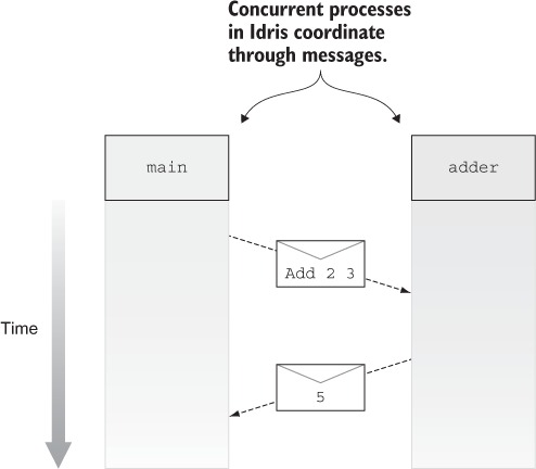
Despite its advantages, however, concurrent programming is notoriously error prone. The need for processes to interact with each other can greatly increase a system’s complexity. For each process, you need to ensure that the messages it sends and
receives are properly coordinated with other processes. If, for example, main and adder aren’t properly coordinated and each is expecting to receive a message from the other at the same time, they’ll deadlock.Types versus testing for concurrent programs
Testing a concurrent program is difficult because, unlike a purely sequential program, there’s no guarantee about the order in which operations from different processes will execute. Even if two processes are correctly coordinated when you run a test once, there’s no guarantee they’ll be correctly coordinated when you next run the test. On the other hand, if you can express the coordination between processes in types, you can be sure that a concurrent program that type-checks has properly coordinated processes.
When you write concurrent programs, you’ll ideally have a model of how processes should interact. Using types, you can make this model explicit in code. Then, if a concurrent program type-checks, you’ll know that it correctly follows the model. In particular, you can do two things:
- Define an interface for adder that describes the form of messages it will handle.
- Define a protocol that defines the order of message passing, ensuring that main will always send a message to adder and then receive a reply, and adder will always do the opposite.
Concurrent programming is an extensive topic, and there are several ways you can use types to model coordination between processes. We’ll look at one example of how to do this in chapter 15.
1.2.4. Type, define, refine: the process of type-driven development
In each of these introductory examples, we’ve discussed in general terms how we might model a system: by describing the valid forms of inputs and outputs for matrix operations, the valid states of an interactive system, or the order of transmission of messages between concurrent processes. In each case, to implement the system, you start by trying to find a type that captures the important details of the model, and then define functions to work with that type, refining the type as necessary.
To put it succinctly, you can characterize type-driven development as an iterative process of type, define, refine: writing a type, implementing a function to satisfy that type, and refining the type or definition as you learn more about the problem.
With matrix addition, for example, you do the following:
- Type— Write a Matrix data type, and use it as the input and output types for an addition function.
- Define— Write an addition function that satisfies its input and output types.
- Refine— Notice that the input and output types for your addition function allow you to give invalid inputs with different dimensions, and then make the type more precise by including the dimensions of the matrices.
1.2.5. Dependent types
In the matrix arithmetic example, we began with a Matrix type and then refined it to include the number of rows and columns. This means, for example, that Matrix 3 4 is the type of 3 × 4 matrices. In this type, 3 and 4 are ordinary values. A dependent type, such as Matrix, is a type that’s calculated from some other values. In other words, it depends on other values.
By including values in a type like this, you can make types as precise as required. For example, some languages have a simple list type, describing lists of objects. You can make this more precise by parameterizing over the element type: a generic list of strings is more precise than a simple list and differs from a list of integers. You can be more precise still with a dependent type: a list of 4 strings differs from a list of 3 strings.
Table 1.2 illustrates how types in Idris can have differing levels of precision even for fundamental operations such as appending lists. Suppose you have two specific input lists of strings:
["a", "b", "c", "d"] ["e", "f", "g"]
Table 1.2. Appending specific typed lists. Unlike simple types, where there’s no difference between the input and output list types, dependent types allow the length to be encoded in the type.
| Input ["a", "b", "c", "d"] | Input ["e", "f", "g"] | Output type | |
|---|---|---|---|
| Simple | AnyList | AnyList | AnyList |
| Generic | List String | List String | List String |
| Dependent | Vect 4 String | Vect 3 String | Vect 7 String |
When you append them, you’ll expect the following output list:
["a", "b", "c", "d", "e", "f", "g"]
Using a simple type, both input lists have type AnyList, as does the output list. Using a generic type, you can specify that the input lists are both lists of strings, as is the output list. The more-precise types mean that, for example, the output is clearly related to the input in that the element type is unchanged. Finally, using a dependent type, you can specify the sizes of the input and output lists. It’s clear from the type that the length of the output list is the sum of the lengths of the input lists. That is, a list of 3 strings appended to a list of 4 strings results in a list of 7 strings.
Lists and vectors
The syntax for the types in table 1.2 is valid Idris syntax. Idris provides several ways of building list types, with varying levels of precision. In the table, you can see two of these, List and Vect. AnyList is included in the table purely for illustrative purposes and is not defined in Idris. List encodes generic lists with no explicit length, and Vect (short for “vector”) encodes lists with the length explicitly in the type. You’ll see much more of both these types throughout this book.
Table 1.3 illustrates how the input and output types of an append function can be written with increasing levels of precision in Idris. Using simple types, you can write the input and output types as AnyList, suggesting that you have no interest in the types of the elements of the list. Using generic types, you can write the input and output types as List elem. Here, elem is a type variable standing for the element types. Because the type variable is the same for both inputs and the output, the types specify that both the input lists and the output list have a consistent element type. If you append two lists of integers, the types guarantee that the output will also be a list of integers. Finally, using dependent types, you can write the inputs as Vect n elem and Vect m elem, where n and m are variables representing the length of each list. The output type specifies that the resulting length will be the sum of the lengths of the inputs.
Table 1.3. Appending typed lists, in general. Type variables describe the relationships between the inputs and outputs, even though the exact inputs and outputs are unknown.
| Input 1 type | Input 2 type | Output type | |
|---|---|---|---|
| Simple | AnyList | AnyList | AnyList |
| Generic | List elem | List elem | List elem |
| Dependent | Vect n elem | Vect m elem | Vect (n + m) elem |
Type variables
Types often contain type variables, like n, m, and elem in table 1.3. These are very much like parameters to generic types in Java or C#, but they’re so common in Idris that they have a very lightweight syntax. In general, concrete type names begin with an uppercase letter, and type variable names begin with a lowercase letter.
In the dependent type for the append function in table 1.3, the parameters n and m are ordinary numeric values, and the + operator is the normal addition operator. All of these could appear in programs just as they’ve appeared here in the types.
Introductory exercises
Throughout this book, exercises will help reinforce the concepts you’ve learned. As a warm-up, take a look at the following selection of function specifications, given purely in the form of input and output types. For each of them, suggest possible operations
that would satisfy the given input and output types. Note that there could be more than one answer in each case.- Input type: Vect n elem Output type: Vect n elem
- Input type: Vect n elem Output type: Vect (n * 2) elem
- Input type: Vect (1 + n) elem Output type: Vect n elem
- Assume that Bounded n represents a number between zero and n - 1. Input types: Bounded n, Vect n elem Output type: elem
1.3. Pure functional programming
Idris is a pure functional programming language, so before we begin exploring Idris in depth, we should look at what it means for a language to be functional, and what we mean by the concept of purity. Unfortunately, there’s no universally agreed-on definition of exactly what it means for a programming language to be functional, but for our purposes we’ll take it to mean the following:
- Programs are composed of functions.
- Program execution consists of the evaluation of functions.
- Functions are a first-class language construct.
This differs from an imperative programming language primarily in that functional programming is concerned with the evaluation of functions, rather than the execution of statements.
In a pure functional language, the following are also true:
- Functions don’t have side effects such as modifying global variables, throwing exceptions, or performing console input or output.
- As a result, for any specific inputs, a function will always give the same result.
You may wonder, very reasonably, how it’s possible to write any useful software under these constraints. In fact, far from making it more difficult to write realistic programs, pure functional programming allows you to treat tricky concepts such as state and exceptions with the respect they deserve. Let’s explore further.
1.3.1. Purity and referential transparency
The key property of a pure function is that the same inputs always produce the same result. This property is known as referential transparency. An expression (such as a function call) in a function is referentially transparent if it can be replaced with its result without changing the behavior of the function. If functions produce only results, with no side effects, this property is clearly true. Referential transparency is a very useful concept in type-driven development, because if a function has no side effects and is
defined entirely by its inputs and outputs, then you can look at its input and output types and have a clear idea of the limits of what the function can do.Figure 1.4 shows example inputs and outputs for the append function. It takes two inputs and produces a result, but there’s no interaction with a user, such as reading from the keyboard, and no informative output, such as logging or progress bars.
Figure 1.4. A pure function, taking inputs and producing outputs with no observable side effects

Figure 1.5 shows pure functions in general. There can be no observable side effects when running these programs, other than perhaps making the computer slightly warmer or taking a different amount of time to run.
Figure 1.5. Pure functions, in general, take only inputs and have no observable side effects.
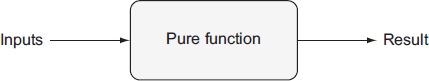
Pure functions are very common in practice, particularly for constructing and manipulating data structures. It’s possible to reason about their behavior because the function always gives the same result for the same inputs; these functions are important components of larger programs. The preceding append function is pure, and it’s a valuable component for any program that works with lists. It produces a list as a result, and because it’s pure, you know that it won’t require any input, output any logging, or do anything destructive like delete files.
1.3.2. Side-effecting programs
Realistically, programs must have side effects in order to be useful, and you’re always going to have to deal with unexpected or erroneous inputs in practical software. At first, this would seem to be impossible in a pure language. There is a way, however: pure functions may not be able to perform side effects, but they can describe them.
Consider a function that reads two lists from a file, appends them, prints the resulting list, and returns it. The following listing outlines this function in imperative-style pseudocode, using simple types.
Listing 1.1. Appending lists read from a file (pseudocode)
List appendFromFile(File h) { list1 = readListFrom(h) list2 = readListFrom(h) result = append(list1, list2) print(result) return result } This program takes a file handle as an input and returns a List with some side effects. It reads two lists from the given file and prints the list before returning. Figure 1.6 illustrates this for the situation when the file contains the two lists ["a", "b", "c", "d"] and ["e", "f", "g"].
Figure 1.6. A side-effecting program, reading inputs from a file, printing the result, and returning the result
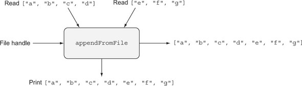
The appendFromFile function doesn’t satisfy the referential transparency property. Referential transparency requires that an expression can be replaced by its result without changing the program’s behavior. Here, however, replacing a call to appendFromFile with its result means that nothing will be read from the file, and nothing will be output to the screen. The function’s input and output types tell us that the input is a file and the output is a list, but nothing in the type describes the side effects the function may execute.
In pure functional programming in general, and Idris in particular, you can solve this problem by writing functions that describe side effects, rather than functions that execute them, and defer the details of execution to the compiler and runtime system. We’ll explore this in greater detail in chapter 5; for now, it’s sufficient to recognize that a program with side effects has a type that makes this explicit. For example, there’s a distinction between the following:
- String is the type of a program that results in a String and is guaranteed to perform no input or output as side effects.
- IO String is the type of a program that describes a sequence of input and output operations that result in a String.
Type-driven development takes this idea much further. As you’ll see from chapter 12 onward, you can define types that describe the specific side effects a program can have, such as console interaction, reading and writing global state, or spawning concurrent processes and sending messages.
1.3.3. Partial and total functions
Idris supports an even stronger property than purity for functions, making a distinction between partial and total functions. A total function is guaranteed to produce a result, meaning that it will return a value in a finite time for every possible well-typed input, and it’s guaranteed not to throw any exceptions. A partial function, on the other hand, might not return a result for some inputs. Here are a couple of examples:- The append function is total for finite lists, because it will always return a new list.
- The function that returns the first element of a list is partial, because it’s not defined if the list is empty, and it will therefore crash.
Total functions and long-running programs
A total function is guaranteed to produce a finite prefix of a potentially infinite result. As you’ll see in chapter 11, you can write command shells or servers as total functions that guarantee a response for every user input, indefinitely.
The distinction is important because knowing that a function is total allows you to make much stronger claims about its behavior based on its type. If you have a function with a return type of String, for example, you can make different claims depending on whether the function is partial or total.
- If it’s total— It will return a value of type String in finite time.
- If it’s partial— If it doesn’t crash or enter an infinite loop, the value it returns will be a String.
In most modern languages, we must assume that functions are partial and can therefore only make the latter, weaker, claim. Idris checks whether functions are total, so we can therefore often make the former, stronger, claim.
The halting problem is the problem of determining whether a program terminates for some specific input. Thanks to Alan Turing, we know that it’s not possible to write a program that solves the halting problem in general. Given this, it’s reasonable to wonder how Idris can determine that a function is total, which is essentially checking that a function terminates for all inputs.
Although it can’t solve the problem in general, Idris can identify a large class of functions that are definitely total. You’ll learn more about how it does so, along with some techniques for writing total functions, in chapters 10 and 11.
A useful pattern in type-driven development is to write a type that precisely describes the valid states of a system (like the ATM in section 1.2.2) and that constrains the operations
the system is allowed to perform. A total function with that type is then guaranteed by the type checker to perform those operations as precisely as the type requires.1.4. A quick tour of Idris
The Idris system consists of an interactive environment and a batch mode compiler. In the interactive environment, you can load and type-check source files, evaluate expressions, search libraries, browse documentation, and compile and run complete programs. We’ll use these features extensively throughout this book.
In this section, I’ll briefly introduce the most important features of the environment, which are evaluation and type checking, and describe how to compile and run Idris programs. I’ll also introduce the two most distinctive features of the Idris language itself:
- Holes, which stand for incomplete programs
- The use of types as first-class language constructs
As you’ll see, by using holes you can define functions incrementally, asking the type checker for contextual information to help complete definitions. Using first-class types, you can be very precise about what a function is intended to do, and even ask the type checker to fill in some of the details of functions for you.
1.4.1. The interactive environment
Much of your interaction with Idris will be through an interactive environment called the read-eval-print loop, typically abbreviated as REPL. As the name suggests, the REPL will read input from the user, usually in the form of an expression, evaluate the expression, and then print the result.
Once Idris is installed, you can start the REPL by typing idris at a shell prompt. You should see something like the following:
____ __ _ / _/___/ /____(_)____ / // __ / ___/ / ___/ Version 1.0 _/ // /_/ / / / (__ ) http://www.idris-lang.org/ /___/\__,_/_/ /_/____/ Type :? for help Idris is free software with ABSOLUTELY NO WARRANTY. For details type :warranty. Idris>
Installing Idris
You can find instructions on how to download and install Idris for Linux, OS X, or Windows in appendix A.
You can enter expressions to be evaluated at the Idris> prompt. For example, arithmetic expressions work in the conventional way, with the usual precedence rules (that is, * and / have higher precedence than + and -):
Idris> 2 + 2 4 : Integer Idris> 2.1 * 20 42.0 : Double Idris> 6 + 8 * 11 94 : IntegerYou can also manipulate Strings. The ++ operator concatenates Strings, and the reverse function reverses a String:
Idris> "Hello" ++ " " ++ "World!" "Hello World!" : String Idris> reverse "abcdefg" "gfedcba" : String
Notice that Idris prints not only the result of evaluating the expression, but also its type. In general, if you see something of the form x : T—some expression x, a colon, and some other expression T—this can be read as “x has type T.” In the previous examples, you have the following:
- 4 has type Integer.
- 42.0 has type Double.
- "Hello World!" has type String.
1.4.2. Checking types
The REPL provides a number of commands, all prefixed by a colon. One of the most commonly useful is :t, which allows you to check the types of expressions without evaluating them:
Idris> :t 2 + 2 2 + 2 : Integer Idris> :t "Hello!" "Hello!" : String
Types, such as Integer and String, can be manipulated just like any other value, so you can check their types too:
Idris> :t Integer Integer : Type Idris> :t String String : Type
It’s natural to wonder what the type of Type itself might be. In practice, you’ll never need to worry about this, but for the sake of completeness, let’s take a look:
Idris> :t Type Type : Type 1That is, Type has type Type 1, Type 1 has type Type 2, and so on forever, as far as we’re concerned. The good news is that Idris will take care of the details for you, and you can always write Type alone.
1.4.3. Compiling and running Idris programs
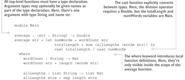
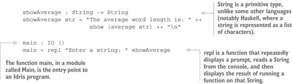
As well as evaluating expressions and inspecting the types of functions, you’ll want to be able to compile and run complete programs. The following listing shows a minimal Idris program.
Listing 1.2. Hello, Idris World! (Hello.idr)
At this stage, there’s no need to worry too much about the syntax or how the program works. For now, you just need to know that Idris source files consist of a module header and a collection of function and data type definitions. They may also import other source files.
Whitespace significance
Whitespace is significant in Idris, so when you type listing 1.2, make sure there are no spaces at the beginning of each line.
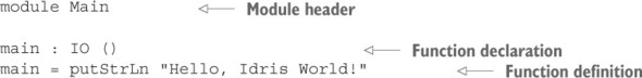
Here, the module is called Main, and there’s only one function definition, called main. The entry point to any Idris program is the main function in the Main module.
To run the program, follow these steps:
- Create a file called Hello.idr in a text editor.[1] Idris source files all have the extension .idr.
I recommend Atom because it has a mode for interactive editing of Idris programs, which we’ll use in this book.1 - Enter the code in listing 1.2.
- In the working directory where you saved Hello.idr, start up an Idris REPL with the command idris Hello.idr.
- At the Idris prompt, type :exec.
If all is well, you should see something like the following:
$ idris Hello.idr ____ __ _ / _/___/ /____(_)____ / // __ / ___/ / ___/ Version 1.0 _/ // /_/ / / / (__ ) http://www.idris-lang.org/ /___/\__,_/_/ /_/____/ Type :? for help Idris is free software with ABSOLUTELY NO WARRANTY. For details type :warranty. Type checking ./Hello.idr *Hello> :exec Hello, Idris WorldHere, $ stands for your shell prompt. Alternatively, you can create a standalone executable by invoking the idris command with the -o option, as follows:
$ idris Hello.idr -o Hello $ ./Hello Hello, Idris World
The REPL prompt
The REPL prompt, by default, tells you the name of the file that’s currently loaded. The Idris> prompt indicates that no file is loaded, whereas the prompt *Hello> indicates that the Hello.idr file is loaded.
1.4.4. Incomplete definitions: working with holes
Earlier, I compared working with types and values to inserting shapes into a shape-sorter toy. Much as the square shape will only fit through a square hole, the argument "Hello, Idris World!" will only fit into a function in a place where a String type is expected.
Idris functions themselves can contain holes, and a function with a hole is incomplete. Only a value of an appropriate type will fit into the hole, just as a square shape will only fit into a square hole in the shape sorter. Here’s an incomplete implementation of the “Hello, Idris World!” program:
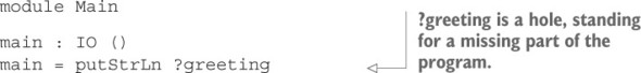
If you edit Hello.idr to replace the string "Hello, Idris World!" with ?greeting and load it into the Idris REPL, you should see something like the following:
Type checking ./Hello.idr Holes: Main.greeting *Hello>
The syntax ?greeting introduces a hole, which is a part of the program yet to be written. You can type-check programs with holes and evaluate them at the REPL.
Here, when Idris encounters the ?greeting hole, it creates a new name, greeting, that has a type but no definition. You can inspect the type using :t at the REPL:
*Hello> :t greeting -------------------------------------- greeting : String
If you try to evaluate it, on the other hand, Idris will show you that it’s a hole:
*Hello> greeting ?greeting : String
Instead of exiting the REPL and restarting, you can also reload Hello.idr with the :r REPL command as follows:
*Hello> :r Type checking ./Hello.idr Holes: Main.greeting *Hello>
Holes allow you to develop programs incrementally, writing the parts you know and asking the machine to help you by identifying the types for the parts you don’t. For example, let’s say you’d like to print a character (with type Char) instead of a String. The putStrLn function requires a String argument, so you can’t simply pass a Char to it.
Listing 1.3. A program with a type error
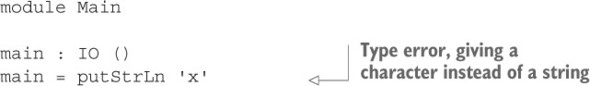
If you try loading this program into the REPL, Idris will report an error:
Hello.idr:4:17:When checking right hand side of main: When checking an application of function Prelude.putStrLn: Type mismatch between Char (Type of 'x') and String (Expected type)
You have to convert a Char to a String somehow. Even if you don’t know exactly how to do this at first, you can start by adding a hole to stand in for a conversion.
module Main main : IO () main = putStrLn (?convert 'x')
Then you can check the type of the convert hole:

The type of the hole, Char -> String, is the type of a function that takes a Char as an input and returns a String as an output. We’ll discuss type conversions in more detail in chapter 2, but an appropriate function to complete this definition is cast:
main : IO () main = putStrLn (cast 'x')
1.4.5. First-class types
A first-class language construct is one that’s treated as a value, with no syntactic restrictions on where it can be used. In other words, a first-class construct can be passed to functions, returned from functions, stored in variables, and so on.In most statically typed languages, there are restrictions on where types can be used, and there’s a strict syntactic separation between types and values. You can’t, for example, say x = int in the body of a Java method or C function. In Idris, there are no such restrictions, and types are first-class; not only can types be used in the same way as any other language construct, but any construct can appear as part of a type.
This means that you can write functions that compute types, and the return type of a function can differ depending on the input value to a function. This idea comes up regularly when programming in Idris, and there are several real-world situations where it’s useful:
- A database schema determines the allowed forms of queries on a database.
- A form on a web page determines the number and type of inputs expected.
- A network protocol description determines the types of values that can be sent or received over a network.
In each of these cases, one piece of data tells you about the expected form of some other data. If you’ve programmed in C, you’ll have seen a similar idea with the printf function, where one argument is a format string that describes the number and expected types of the remaining arguments. The C type system can’t check that the format string is consistent with the arguments, so this check is often hardcoded into C compilers. In Idris, however, you can write a function similar to printf directly, by taking advantage of types as first-class constructs. You’ll see this specific example in chapter 6.
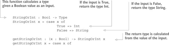
The following listing illustrates the concept of first-class types with a small example: computing a type from a Boolean input.
Listing 1.4. Calculating a type, given a Boolean value (FCTypes.idr)
We’ll go into much more detail on Idris syntax in the coming chapters. For now, just keep the following in mind:
- A function type takes the form a -> b -> ... -> t, where a, b, and so on, are the input types, and t is the output type. Inputs may also be annotated with names, taking the form (x : a) -> (y : b) -> ... -> t.
- name : type declares a new function, name, of type type.
- Functions are defined by equations: square x = x * x
This defines a function called square that multiplies its input by itself
Here, StringOrInt is a function that computes a type. Listing 1.4 uses it in two ways:
- In getStringOrInt, StringOrInt calculates the return type. If the input is True, getStringOrInt returns an Int; otherwise it returns a String.
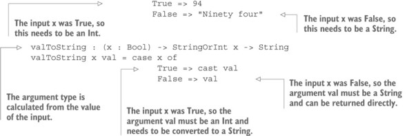
- In valToString, StringOrInt calculates an argument type. If the first input is True, the second input must be an Int; otherwise it must be a String.
You can see in detail what’s going on by introducing holes in the definition of valToString:
valToString : (x : Bool) -> StringOrInt x -> String valToString x val = case x of True => ?xtrueType False => ?xfalseType
Inspecting the type of a hole with :t gives you not only the type of the hole itself, but also the types of any local variables in scope. If you check the type of xtrueType, you’ll see the type of val, which is computed when x is known to be True:
*FCTypes> :t xtrueType x : Bool val : Int -------------------------------------- xtrueType : String
So, if x is True, then val must be an Int, as computed by the StringOrInt function. Similarly, you can check the type of xfalseType to see the type of val when x is known to be False:
*FCTypes> :t xfalseType x : Bool val : String -------------------------------------- xfalseType : String
This is a small example, but it illustrates a fundamental concept of type-driven development and programming with dependent types: the idea that the type of a variable can be computed from the value of another. In each case, Idris has used StringOrInt to refine the type of val, given what it knows about the value of x.
1.5. Summary
- Types are a means of classifying values. Programming languages use types to decide how to lay out data in memory, and to ensure that data is interpreted consistently.
- A type can be viewed as a specification, so that a language implementation (specifically, its type checker) can check whether a program conforms to that specification.
- Type-driven development is an iterative process of type, define, refine, creating a type to model a system, then defining functions, and finally refining the types as necessary.
- In type-driven development, a type is viewed more like a plan, helping an interactive environment guide the programmer to a working program.
- Dependent types allow you to give more-precise types to programs, and hence more informative plans to the machine.
- In a functional programming language, program execution consists of evaluating functions.
- In a purely functional programming language, additionally, functions have no side effects.
- Instead of writing programs that perform side effects, you can write programs that describe side effects, with the side effects stated explicitly in a program’s type.
- A total function is guaranteed to produce a result for any well-typed input in finite time.
- Idris is a programming language that’s specifically designed to support type-driven development. It’s a purely functional programming language with first-class dependent types.
- Idris allows programs to contain holes that stand for incomplete programs.
- In Idris, types are first-class, meaning that they can be stored in variables, passed to functions, or returned from functions like any other value.
Chapter 2. Getting started with Idris
This chapter covers
- Using built-in types and functions
- Defining functions
- Structuring Idris programs
When learning any new language, it’s important to have a solid grasp of the fundamentals before moving on to the more distinctive features of the language. With this in mind, before we begin exploring dependent types and type-driven development itself, we’ll look at some types and values that will be familiar to you from other languages, and you’ll see how they work in Idris. You’ll also see how to define functions and put these together to build a complete, if simple, Idris program.
If you’re already familiar with a pure functional language, particularly Haskell, much of this chapter will seem very familiar. Listing 2.1 shows a simple, but self--contained, Idris program that repeatedly prompts for input from the console and then displays the average length of the words in the input. If you’re already comfortable reading this program with the help of the annotations, you can safely skip this chapter, as it deliberately avoids introducing any language features specific to Idris.[1]
Even so, I still suggest you browse through this chapter’s tips and notes and read the summary at the end to make sure there aren’t any small details you’ve missed.Comparing Idris to Haskell, the most important difference is that Idris doesn’t use lazy evaluation by default.
1
Otherwise, don’t worry. By the end of this chapter we’ll have covered all of the necessary features for you to be able to implement similar programs yourself.
Listing 2.1. A complete Idris program to calculate average word length (Average.idr)
2.1. Basic types
Idris provides some standard basic types and functions for working with various forms, characters, and strings. In this section, I’ll give you an overview of these, along with some examples. These basic types are defined in the Prelude, which is a collection of standard types and functions automatically imported by every Idris program.
I’ll show you several example expressions in this section, and it may seem fairly clear what they should do. Nevertheless, instead of simply reading them and nodding, I strongly recommending you type the examples at the Idris REPL. You’ll learn the syntax much more easily by using it than you will by merely reading it.
Along the way, we’ll also encounter a couple of useful REPL features that will allow us to store the results of calculations at the REPL.
The Prelude
The types and functions I’ll discuss are defined in the Prelude. The Prelude is Idris’s standard library, always available at the REPL and automatically imported by every Idris program. With the exception of some primitive types and operations, everything in the Prelude is written in Idris itself.2.1.1. Numeric types and values
Idris provides several basic numeric types, including the following:
- Int—A fixed-width signed integer type. It’s guaranteed to be at least 31 bits wide, but the exact width is system dependent.
- Integer—An unbounded signed integer type. Unlike Int, there’s no limit to the size of the numbers that can be represented, other than your machine’s memory, but this type is more expensive in terms of performance and memory usage.
- Nat—An unbounded unsigned integer type. This is very often used for sizes and indexing of data structures, because they can never be negative. You’ll see much more of Nat later.
- Double—A double-precision floating-point type.
Subtraction with Nats
Because Nats can never be negative, a Nat can only be subtracted from a larger Nat.
We can use standard numeric literals as values for each of these types. For example, the literal 333 can be of type Int, Integer, Nat, or Double. The literal 333.0 can be only of type Double, due to the explicit decimal point.
You can try some simple calculations at the REPL:
Idris> 6 + 3 * 12 42 : Integer Idris> 6.0 + 3 * 12 42.0 : Double
Note that Idris will treat a number as an Integer by default, unless there’s some context, and both operands must be the same type. Therefore, in the second of the two preceding expressions, the literal 6.0 can be only a Double, so the whole expression is a Double, and 3 and 12 are also treated as Doubles.
The most recent result at the REPL can always be retrieved and used in further calculations by using the special value it:
Idris> 6 + 3 * 12 42 : Integer Idris> it * 2 84 : Integer
It’s also possible to bind expressions to names at the REPL using the :let command:
Idris> :let x = 100 Idris> x 100 : Integer Idris> :let y = 200.0 Idris> y 200.0 : Double
When an expression, such as 6 + 3 * 12, can be one of several types, you can make the type explicit with the notation the <type><expression>, to say that type is the required type of expression:
Idris> 6 + 3 * 12 42 : Integer Idris> the Int (6 + 3 * 12) 42 : Int Idris> the Double (6 + 3 * 12) 42.0 : Double
“the” expressions
the is not built-in syntax but an ordinary Idris function, defined in the Prelude, which takes advantage of first-class types.2.1.2. Type conversions using cast
Arithmetic operators work on any numeric types, but both inputs and the output must have the same type. Sometimes, therefore, you’ll need to convert between types.
Let’s say you’ve defined an Integer and a Double at the REPL:
Idris> :let integerval = 6 * 6 Idris> :let doubleval = 0.1 Idris> integerval 36 : Integer Idris> doubleval 0.1 : Double
If you try to add integerval and doubleval, Idris will complain that they aren’t the same type:
Idris> integerval + doubleval (input):1:8-9:When checking an application of function Prelude.Classes.+: Type mismatch between Double (Type of doubleval) and Integer (Expected type)
To fix this, you can use the cast function, which converts its input to the required type, as long as that conversion is valid. Here, you can cast the Integer to a Double:
Idris> cast integerval + doubleval 36.1 : Double
Idris supports casting between all the primitive types, and it’s possible to add user-defined casts, as you’ll see in chapter 7. Note that some casts may lose information, such as casting a Double to an Integer.
You can also use the to specify which type you want to cast to, as in these examples:
Idris> the Integer (cast 9.9) 9 : Integer Idris> the Double (cast (4 + 4)) 8.0 : Double
2.1.3. Characters and strings
Idris also provides Unicode characters and strings as primitive types, along with some useful primitive functions for manipulating them.- Character literals (of type Char) are enclosed in single quotation marks, such as 'a'.
- String literals (of type String) are enclosed in double quotation marks, such as "Hello world!"
Like many other languages, Idris supports special characters in character and string literals by using escape sequences, beginning with a backslash. For example, a newline character is indicated using \n:
Idris> :t '\n' '\n' : Char Idris> :t "Hello world!\n" "Hello world!\n" : String
These are the most common escape sequences:
- \' for a literal single quote
- \" for a literal double quote
- \\ for a literal backslash
- \n for a newline character
- \t for a tab character
The Prelude defines several useful functions for manipulating Strings. You can see some of these in action at the REPL:
Idris> length "Hello!" 6 : Nat Idris> reverse "drawer" "reward" : String Idris> substr 6 5 "Hello world" "world" : String Idris> "Hello" ++ " " ++ "World" "Hello World" : String
Here’s a brief explanation of these functions:
- length—Gives the length of its argument as a Nat because a String can’t have a negative length
- reverse—Returns a reversed version of its input
- substr—Returns a substring of an input string, given a position to start at and the desired length of the substring
- ++—An operator that concatenates two Strings
Idris> length ("Hello" ++ " " ++ "World") 11 : Nat Function syntax
Calling functions by separating the arguments with spaces may seem strange at first. There’s a good reason for it, though, as you’ll discover when we look at function types later in this chapter. In short, it makes manipulating functions much more flexible.
2.1.4. Booleans
Idris provides a Bool type for representing truth values. A Bool can take the value True or False. The operators && and || represent logical and and or, respectively:
Idris> True && False False : Bool Idris> True || False True : Bool
The usual comparison operators (<, <=, ==, /=, >, >=) are available:
Idris> 3 > 2 True : Bool Idris> 100 == 99 False : Bool Idris> 100 /= 99 True : Bool
Inequality
The inequality operator in Idris is /=, which follows Haskell syntax, rather than !=, which would follow the syntax of languages like C and Java.
There is also an if...then...else construct. This is an expression, so it must always include both a then branch and an else branch. For example, you can write an expression that evaluates to a different message as a String, depending on the length of a word:
Idris> :let word = "programming" Idris> if length word > 10 then "What a long word!" else "Short word" "What a long word!" : String
2.2. Functions: the building blocks of Idris programs
Now that you’ve seen some basic types and a simple control structure, you can begin defining functions. In this section, you’ll write some Idris functions using the basic types you’ve seen so far, load them into the Idris system, and test them at the REPL. You’ll also see how the functional programming style allows you to write more generic programs in two ways:
- Using variables in function types, so that functions can be written to work with several different types
- Using higher-order functions to capture common programming patterns
2.2.1. Function types and definitions
Function types are composed of one or more input types and an output type. For example, a function that takes an Int as input and returns another Int would be written as Int -> Int. The following listing shows a simple function definition with this type, the double function.
Listing 2.2. A function to double an Int (Double.idr)
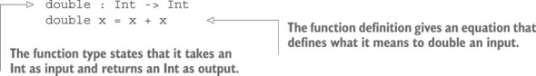
You can try this function by typing it into a file, Double.idr; loading it into the Idris REPL by typing idris Double.idr at the shell prompt; and then trying some examples at the REPL:
*Double> double 47 94 : Int *Double> double (double 15) 60 : Int
Figure 2.1 shows the components of this function definition. All functions in Idris, like double, are introduced with a type declaration and then defined by equations with a left side and a right side.
Figure 2.1. The components of a function definition
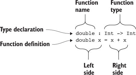
An expression is evaluated by rewriting the expression according to these equations until no further rewriting can be done. Functions, therefore, define rules by which expressions can be rewritten. For example, consider the definition of double:
double x = x + x
This means that whenever the Idris evaluator encounters an expression of the form double x, with some expression standing for x, it should be rewritten as x + x.
So, in the example double (double 15),
- First, the inner double 15 is rewritten as 15 + 15.
- 15 + 15 is rewritten as 30.
- double 30 is rewritten as 30 + 30.
- 30 + 30 is rewritten as 60.
You might have noticed that instead of choosing to evaluate the inner double 15 first, you could have chosen the outer double (double 15), which would have reduced to double 15 + double 15. Either order is possible, and each would lead to the same result. Idris, by default, will evaluate the innermost expression first. In other words, it will evaluate function arguments before function definitions.
There are merits and drawbacks to both choices, and as a result this topic has been debated at length! Now is not the time to revisit this debate, but if you’re interested, you can investigate lazy evaluation. Idris supports lazy evaluation using explicit types, as you’ll see in chapter 11.
Optionally, you can give explicit names in the input types of a function. For example, you could write the type of double as follows:
double : (value : Int) -> Int
This has exactly the same meaning as the previous declaration (double : Int -> Int). There are two reasons why you might make the names of the arguments explicit:
- Naming the argument in the type can give the reader some information about the purpose of the argument.
- Naming the argument means you can refer to it later.
You’ll see more of this in chapter 4 when we begin to explore dependent types in depth. For now, remember the example of first-class types from chapter 1, where I gave the following Idris type for getStringOrInt:
getStringOrInt : (x : Bool) -> StringOrInt x
The first argument, of type Bool, was given the name x, which then appears in the return type.
Type declarations are required!
Functions in Idris must have an explicit type declaration, like double : Int -> Int here. Some other functional languages, most notably Haskell and ML, allow programmers to omit type declarations and have the compiler infer the type. In a language with first-class types, however, this generally turns out to be impossible. In any case, it’s
undesirable to omit type declarations in type-driven development. Our philosophy is to use types to help us write programs, rather than to use programs to help us infer types!2.2.2. Partially applying functions
When a function has more than one argument, you can create a specialized version of the function by omitting the later arguments. This is called partial application.
For example, assume you have an add function that adds two integers, defined as follows in the Partial.idr file:
add : Int -> Int -> Int add x y = x + y
If you apply the function to two arguments, it will evaluate to an Int:
*Partial> add 2 3 5 : Int
If, on the other hand, you only apply the function to one argument, omitting the second, Idris will return a function of type Int -> Int:
*Partial> add 2 add 2 : Int -> Int
By applying add to only one argument, you’ve created a new specialized function, add 2, that adds 2 to its argument. You can see this more explicitly by creating a new function with :let:
*Partial> :let addTwo = add 2 *Partial> :t addTwo addTwo : Int -> Int *Partial> addTwo 3 5 : Int
The function application syntax, applying functions to arguments simply by separating the function from the argument with whitespace, gives a particularly concise syntax for partial application. Partial application is common in Idris programs, and you’ll see some examples of it in action shortly, in section 2.2.5.
2.2.3. Writing generic functions: variables in types
As well as concrete types, such as Int, String, and Bool, function types can contain variables. Variables in a function type can be instantiated with different values, just like variables in functions themselves.
For example, let’s consider the identity function, which returns its input, unchanged. The identity function on Ints is written as follows:
identityInt : Int -> Int identityInt x = x
Similarly, the identity function on Strings is written like this:
identityString : String -> String identityString x = x
And here’s the identity function on Bools:
identityBool : Bool -> Bool identityBool x = x
You may have noticed a pattern here. In each case the definition is the same! You don’t need to know anything about x because you’re returning it unchanged in each case. So, instead of writing an identity function for every type separately, you can write one identity function using a variable, ty, at the type level, in place of a concrete type:
identity : ty -> ty identity x = x
The id function
In fact, there is an identity function in the Prelude called id, defined in exactly the same way as identity here.
The ty in the type of identity is a variable, standing for any type. Therefore, identity can be called with any input type, and will return an output with the same type as the input.
Variable names in types
Any name that appears in a type declaration, begins with a lowercase letter, and is otherwise undefined is assumed to be a variable. Note that I’m careful to call these variables, rather than type variables. This is because, with dependent types, variables in types don’t necessarily stand for only types, as you’ll see in chapter 3.
You’ve already seen a form of the identity function when working with numeric types: the is an identity function. It’s defined in the Prelude as follows:
the : (ty : Type) -> ty -> ty the ty x = x
It takes an explicit type as its first argument, which is explicitly named ty. The type of the second argument is given by the input value of the first argument. This is a simple example of dependent types in action, in that the value of an earlier argument gives the type of a later argument. You can see this explicitly at the REPL, by partially applying the to only one argument:
Idris> :t the Int the Int : Int -> Int Idris> :t the String the String : String -> String Idris> :t the Bool the Bool : Bool -> Bool
2.2.4. Writing generic functions with constrained types
The first function you saw in section 2.2.1, double, doubles the Int given as input:double : Int -> Int double x = x + x
But what about other numeric types? For example, you could also write a function to double a Nat, or an Integer:
doubleNat : Nat -> Nat doubleNat x = x + x doubleInteger : Integer -> Integer doubleInteger x = x + x
As with identity, you’re probably starting to see a pattern here, so let’s see what happens if we try to replace the input and output types with a variable. Put the following in a file called Generic.idr and load it into Idris:
double : ty -> ty double x = x + x
You’ll find that Idris rejects this definition, with the following error message:
Generic.idr:2:8: When checking right hand side of double with expected type ty ty is not a numeric type
The problem is that, unlike identity, double needs to know something about its input x, specifically that it’s numeric. You can only use arithmetic operators on numeric types, so you need to constrain ty so that it only stands for numeric types. The following listing shows how you can do this.
Listing 2.3. A generic type, constrained to numeric types (Generic.idr)
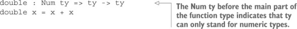
The type Num ty => ty -> ty can be read as, “A function with input type ty and output type ty under the constraint that ty is a numeric type.”
Type constraints
Constraints on generic types can be user-defined using interfaces, which we’ll cover in depth in chapter 7. Here, Num is an interface provided by Idris. Interfaces can be given implementations for specific types, and the Num interface has implementations for numeric types.
Perhaps surprisingly, arithmetic and comparison operators aren’t primitive operators in Idris, but rather functions with constrained generic types. Infix operators such as +,
==, and <= are really functions with two inputs, as you can see by checking their types at the REPL:Idris> :t (+) (+) : Num ty => ty -> ty -> ty Idris> :t (==) (==) : Eq ty => ty -> ty -> Bool Idris> :t (<=) (<=) : Ord ty => ty -> ty -> Bool
As well as Num for numeric types, here you can see two other constraints provided by Idris:
- Eq states that the type must support the equality and inequality operators, == and /=.
- Ord states that the type must support the comparison operators <, <=, >, and >=.
Infix operators in Idris aren’t a primitive part of the syntax, but are defined by functions. Putting operators in brackets, as with (+), (==), and (<=) in the REPL example, means that they’ll be treated as ordinary function syntax. For example, you can apply (+) to one argument:
Idris> :t (+) 2 (+) 2 : Integer -> Integer
Infix operators can also be partially applied using operator sections:
- (< 3) gives a function that returns whether its input is less than 3.
- (3 <) gives a function that returns whether 3 is less than its input.
An operator in brackets with only one argument is therefore considered to be a function that expects the other missing argument.
2.2.5. Higher-order function types
There are no restrictions on what the argument or return types of a function can be. You’ve already seen how functions of multiple arguments are really functions that return something with a function type. Similarly, functions can take functions as arguments. Such functions are called higher-order functions.
Higher-order functions can be used to create abstractions for repeated programming patterns. For example, say you’ve defined a quadruple function that quadruples its input for any number, using double:
quadruple : Num a => a -> a quadruple x = double (double x)
Or say you have a Shape type that represents any geometric shape, and a function rotate : Shape -> Shape that rotates a shape through 90 degrees. You could define a turn_around function that rotates a shape through 180 degrees as follows:
turn_around : Shape -> Shape turn_around x = rotate (rotate x)
Each of these functions has exactly the same pattern, but they work on different input types. You can capture this pattern using a higher-order function to apply a function to an argument twice. The next listing gives a definition of a twice function, along with new definitions of quadruple and rotate.
Listing 2.4. Defining quadruple and rotate using a higher-order function (HOF.idr)
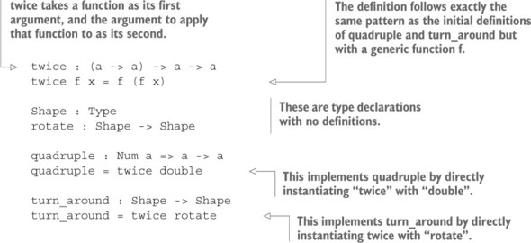
In chapter 1, I introduced the concept of “holes,” which are incomplete function definitions. The type declarations with no definitions in listing 2.4, Shape and rotate, are treated as holes. They allow you to try an idea (such as how to implement turn_around in terms of rotate) without fully defining the types and functions.
In listing 2.4, quadruple and turn_around have function types, Num a => a -> a and Shape -> Shape, respectively, but in their definitions neither has an argument.
The only requirement when checking a definition is that both sides of the definition must have the same type. You can check that this is the case here by looking at the types of the left and right sides of the definition at the REPL. You have the following definition:
turn_around = twice rotateBy checking the types at the REPL, you can see that both turn_around and twice rotate have the same type:
Idris> :t turn_around turn_around : Shape -> Shape Idris> :t twice rotate twice rotate : Shape -> Shape
The definitions of quadruple and turn_around both use partial application, as described in section 2.2.2.
Another common use of partial application is in constructing arguments for higher-order functions. Consider this example, using HOF.idr and adding the definition of add from section 2.2.2:
*HOF> twice (add 5) 10 20 : Int
This uses a partial application of the add function to add 5 to an Int, twice. Because twice requires a function of one argument, and add takes two arguments, you can apply add to one argument so that it’s usable in an application of twice.
You could also use an operator section, as described at the end of section 2.2.4:
*HOF> twice (5 +) 10 20 : Integer
Note that, in the absence of any other type information, Idris has defaulted to Integer, as described in section 2.1.1.
2.2.6. Anonymous functions
When using higher-order functions, it’s often useful to pass an anonymous function as an argument. An anonymous function is generally a small function that you only expect to use once, so there’s no need to create a top-level definition for it.
For example, you could pass an anonymous function that squares its input to twice:
*HOF> twice (\x => x * x) 2 16 : Integer
Anonymous functions are introduced with a backslash \ followed by a list of arguments. If you check the type of the preceding anonymous function, you’ll see that it has a function type:
*HOF> :t \x => x * x \x => x * x : Integer -> Integer
Anonymous functions can take more than one argument, and arguments can optionally be given explicit types:
*HOF> :t \x : Int, y : Int => x + y \x, y => x + y : Int -> Int -> IntNote that the output doesn’t show the types explicitly.
2.2.7. Local definitions: let and where
As functions get larger, it’s usually a good idea to break them down into smaller definitions. Idris provides two constructs for locally defining variables and functions: let and where.
Figure 2.2 illustrates the syntax for let bindings, which define local variables.
If you evaluate this expression at the REPL, you’ll see the following:
Idris> let x = 50 in x + x 100 : Integer
Figure 2.2. A local variable definition: in the expression after the in keyword, x has the value 50.
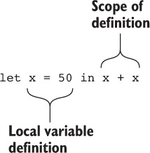
The next listing shows a larger example of let in action. It defines a function, longer, that takes two Strings and returns the length of the longer one. It uses let to record the length of each input.
Listing 2.5. Local variables with let (Let_Where.idr)
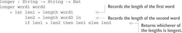
Multiple lets
There can be several definitions in a let block. In listing 2.5, for example, there are two local variables defined in the let block in longer.
Whereas let blocks contain local variable definitions, where blocks contain local function definitions. Listing 2.6 shows where in action. It defines a function to calculate the length of the hypotenuse of a triangle, using the Pythagorean Theorem and a local square function.
Listing 2.6. Local function definitions with where (Let_Where.idr)
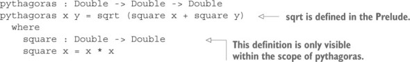
2.3. Composite types
Composite types are composed of other types. In this section, we’ll look at two of the most common composite types provided by Idris: tuples and lists.
2.3.1. Tuples
A tuple is a fixed-size collection, where each value in the collection can have a different type. For example, a pair of an Integer and a String can be written as follows:
Idris> (94, "Pages") (94, "Pages") : (Integer, String)
Tuples are written as a bracketed, comma-separated list of values. Notice that the type of the pair (94, "Pages") is (Integer, String). Tuple types are written using the same syntax as tuple values.
The fst and snd functions extract the first and second items, respectively, from a pair:
Idris> :let mypair = (94, "Pages") Idris> fst mypair 94 : Integer Idris> snd mypair "Pages" : String
Both fst and snd have generic types, because pairs can contain any types. You can check the type of each at the REPL:
Idris> :t fst fst : (a, b) -> a Idris> :t snd snd : (a, b) -> b
You can read the type of fst, for example, as “Given a pair of an a and a b, return the value that has type a.” In these types, you know that both a and b are variables because they begin with lowercase letters.
Tuples can have any number of components, including zero:
Idris> ('x', 8, String) ('x', 8, String) : (Char, Integer, Type) Idris> () () : () The empty tuple, (), is often referred to as “unit” and its type as “the unit type.” Notice that the syntax is overloaded, and Idris will decide whether () means unit or the unit type from the context.
- Types are blue.
- Values (more precisely, data constructors, as I’ll explain in chapter 3) are red.
- Functions are green.
- Variables are magenta.
If these colors aren’t to your liking or are hard to distinguish (for example, if you’re color blind), you can change the settings with the :colour command.
Tuples can also be arbitrarily deeply nested:
Idris> (('x', 8), (String, 'y', 100), "Hello") (('x', 8), (String, 'y', 100), "Hello") : ((Char, Integer), (Type, Char, Integer), String) Internally, all tuples other than the empty tuple are stored as nested pairs. That is, if you write (1, 2, 3, 4), Idris will treat this in the same way as (1, (2, (3, 4))). The REPL will always display a tuple in the non-nested form:
Idris> (1, (2, (3, 4))) (1, 2, 3, 4) : (Integer, Integer, Integer, Integer)
2.3.2. Lists
Lists, like tuples, are collections of values. Unlike tuples, lists can be any size, but every element must have the same type. Lists are written as comma-separated lists of values in square brackets, as follows.
Idris> [1, 2, 3, 4] [1, 2, 3, 4] : List Integer Idris> ["One", "Two", "Three", "Four"] ["One", "Two", "Three", "Four"] : List String
The type of each of these expressions, List Integer and List String, indicates the element type that Idris has inferred for the list. In type-driven development, we typically give types first, and then write a corresponding value or function that satisfies this type. At the REPL, it would be inconvenient to do this for every value, so Idris will try to infer a type for the given value. Unfortunately, it’s not always possible. For example, if you give it an empty list, Idris doesn’t know what the element type should be:
Idris> [] (input):Can't infer argument elem to []
This error message means that Idris can’t work out the element type (which happens to be named elem) for the empty list []. The problem can be resolved in this case by giving an explicit type, using the:
Idris> the (List Int) [] [] : List Int
Like strings, lists can be concatenated with the ++ operator, provided that both operands have the same element type:
Idris> [1, 2, 3] ++ [4, 5, 6, 7] [1, 2, 3, 4, 5, 6, 7] : List Integer
You can add an element to the front of a list using the :: (pronounced “cons”) operator:
Idris> 1 :: [2, 3, 4] [1, 2, 3, 4] : List Integer Idris> 1 :: 2 :: 3 :: 4 :: [] [1, 2, 3, 4] : List Integer
The :: operator is the primitive operator for constructing lists from a head element and a tail, and Nil is a primitive name for the empty list. A list can therefore take one of the following two canonical forms:
- Nil, the empty list
- x :: xs, where x is an element, and xs is another list
Because this can get quite verbose, Idris provides syntactic sugar for lists. List literals consisting of comma-separated elements inside square brackets are desugared to these primitive forms. For example, [] is desugared directly to Nil, and [1, 2, 3] is desugared to 1 :: (2 :: (3 :: Nil)).
There’s also a more concise notation for ranges of numbers. Here are a few examples:
- [1..5] expands to the list [1, 2, 3, 4, 5].
- [1,3..9] expands to the list [1, 3, 5, 7, 9].
- [5,4..1] expands to the list [5, 4, 3, 2, 1].
More generally, [n..m] gives an increasing list of numbers between n and m, and [n,m..p] gives a list of numbers between n and p with the step given by the difference between n and m.
2.3.3. Functions with lists
We’ll discuss lists in more depth in the next chapter, including how to define functions over lists, but there are several useful functions defined in the Prelude. Let’s take a look at some of these.The words function, of type String -> List String, converts a string into a list of the whitespace-separated components of the string:[2]
The words name comes from a similar function in the Haskell libraries. Many Idris function names follow Haskell terminology.
2
Idris> words "'Twas brillig, and the slithy toves" ["'Twas", "brillig,", "and", "the", "slithy", "toves"] : List String
The unwords function, of type List String -> String, does the opposite, converting a list of words into a string where the words are separated by a space:
Idris> unwords ["One", "two", "three", "four!"] "One two three four!" : String
You’ve already seen a length function for calculating the lengths of strings. There’s also an overloaded length function, of type List a -> Nat, that gives the length of a list:
Idris> length ["One", "two", "three", "four!"] 4 : Nat
You can use length and words to write a word-count function for strings:
wordCount : String -> Nat wordCount str = length (words str)
The map function is a higher-order function that applies a function to every element in a list. It has the type (a -> b) -> List a -> List b. This example finds the lengths of every word in a list:
Idris> map length (words "How long are these words?") [3, 4, 3, 5, 6] : List Nat
You can use map and length to write a function that gets the length of every element in a list of Strings:
allLengths : List String -> List Nat allLengths strs = map length strs
If you check the type of map at the REPL, you’ll see something slightly different:
Idris> :t map map : Functor f => (a -> b) -> f a -> f b
The reason for this is that map can work on a variety of structures, not just lists, so it has a constrained generic type. You’ll learn about Functor in chapter 7, but for the moment it’s fine to read f as List in this type.
The filter function is another higher-order function that filters a list according to a Boolean function. It has type (a -> Bool) -> List a -> List a and returns a new list of everything in the input list for which the function returns True. For example, here’s how you find all the numbers larger than 10 in a list:
Idris> filter (> 10) [1,11,2,12,3,13,4,14] [11, 12, 13, 14] : List Integer
You’ve seen the length function on both strings and lists. This works because Idris allows function names to be overloaded to work on multiple types. You can see what’s happening by checking the type of length at the REPL:
*lists> :t length Prelude.List.length : List a -> Nat Prelude.Strings.length : String -> Nat
In fact, there are two functions called length. The prefixes Prelude.List and Prelude.Strings are the namespaces these functions are defined in. Idris decides which length function is required from the context in which it’s used.
The sum function, of type Num a => List a -> a, calculates the sum of a list of numbers:
Idris> sum [1..100] 5050 : Integer
The type of sum states that every element of the input List must have the same type, a, and that type is constrained by Num.
You now know enough to be able to define a function named average that computes the average length of the words in a string. This function is defined in the next listing, which shows the complete Idris file Average.idr.
Listing 2.7. Calculating the average word length in a string (Average.idr)
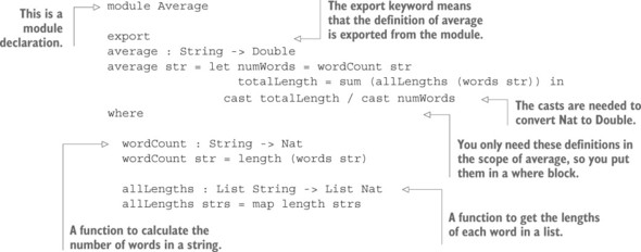
Listing 2.7 also introduces the module and export keywords. A module declaration can optionally be put at the top of a file. This declares a namespace in which every function is defined. Conventionally, module names are the same as the filename (without the .idr extension). The export keyword allows the average function to be used by other modules that import Average.idr.
As usual, you can try this at the REPL by loading Average.idr into Idris, and evaluating as follows:
*Average> average "How long are these words?" 4.2 : Double
By adding a module declaration to the top of Average.idr, you declare a namespace for the definitions in the module. Here, it means that the fully qualified name of the average function is Average.average. A module declaration must be the first thing in the file. If there’s no declaration, Idris calls the module Main.
Modules allow you to divide larger Idris programs logically into several source files, each with their own purpose. They can be imported with an import statement. For example:
- import Average will import the definitions from Average.idr, provided that Average.idr is either in the current directory or in some other path that Idris can find.
- import Utils.Average will import the definitions from Average.idr in a subdirectory called Utils, provided that the file and subdirectory exist.
Modules themselves can be combined into packages and distributed separately. Technically, the Prelude is defined in a module called Prelude, which itself imports several other modules, and which is part of a package called prelude. You can learn more about packages and how to create your own from the Idris package documentation at http://idris-lang.org/documentation/packages.
2.4. A complete Idris program
So far, you’ve seen how to write functions with built-in types and some basic operations on those types. Functions are the basic building blocks of Idris programs, so now that you’ve written some simple functions, it’s time to see how to put these together to build a complete program.2.4.1. Whitespace significance: the layout rule
Whitespace, specifically indentation, is significant in Idris programs. Unlike some other languages, there are no braces or semicolons to indicate where expressions, type declarations, and definitions begin and end. Instead, in any list of definitions and declarations, all must begin in precisely the same column. Listing 2.8 illustrates where definitions and declarations begin and end according to this rule in a file containing the previous definition of average.
Spaces and tabs
One complication with whitespace significance is that tab sizes can be set differently in different editors, and Idris expects tabs and spaces to be used consistently. To avoid any confusion with tab sizes, I strongly recommend you set your editor to replace tabs with spaces!
Listing 2.8. The layout rule applied to average (Average.idr)
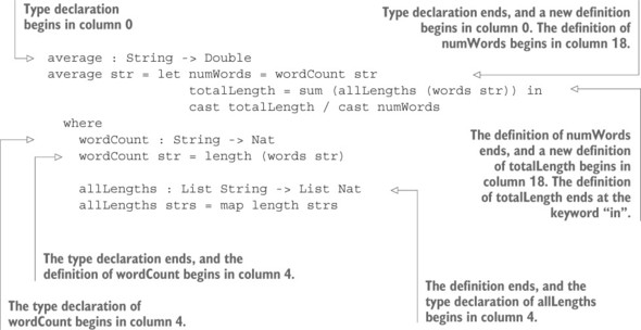
If, for example, allLengths was indented one extra space, as in listing 2.9, it would be considered a continuation of the previous definition of wordCount, and would therefore be invalid.
Listing 2.9. The layout rule, applied incorrectly
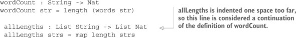
2.4.2. Documentation comments
As with any other language, it’s good form to comment definitions to give the reader of the code an idea of the purposes of functions and document how they work. Idris provides three kinds of comments:- Single-line comments, introduced with -- (two minus signs). These comments continue to the end of the line.
- Multiline nested comments, introduced with {- and ending with -}.
- Documentation comments, which are used to provide documentation for functions and types at the REPL.
The first two types of comments are conventional, and merely cause the commented section to be ignored (the syntax is identical to the syntax of comments in Haskell).
Documentation comments, on the other hand, make documentation available at the REPL, accessible with the :doc command. You can look at the documentation for some of the types and functions we’ve encountered so far. For example, :doc fst produces the following output:
Idris> :doc fst Prelude.Basics.fst : (a, b) -> a Return the first element of a pair. The function is Total
This output includes the fully qualified name of fst, showing that it is defined in the module Prelude.Basics, and states that the function is total, meaning that it’s guaranteed to produce a result for all inputs.
You can also get documentation for types. For example, :doc List gives the following output:
Idris> :doc List Data type Prelude.List.List : Type -> Type Generic lists Constructors: Nil : List elem The empty list (::) : elem -> List elem -> List elem A non-empty list, consisting of a head element and the rest of the list. infixr 7Again, this gives the fully qualified name of the type Prelude.List.List. It also gives the constructors, which are the primitive ways of constructing lists. Finally, for the :: operator, it gives the fixity, which states the operator is right associative (infixr) and has precedence level 7. I’ll describe precedence and the associativity of operators in more detail in chapter 3.
Documentation comments, which produce this documentation, are introduced with three vertical bars, |||. For example, you could document average as follows:
||| Calculate the average length of words in a string. average : String -> Double
Then, :doc average would produce the following output:
*Average> :doc average Average.average : (str : String) -> Double Calculate the average length of words in a string. The function is Total
You can refer to the argument of average by giving it a name, str, and referring to that name in the comment with @str:
||| Calculate the average length of words in a string. ||| @str a string containing words separated by whitespace. average : (str : String) -> Double average str = let numWords = wordCount str totalLength = sum (allLengths (words str)) in cast totalLength / cast numWords
This makes :doc average produce some more informative output:
*Average> :doc average Main.average : (str : String) -> Double Calculate the average length of words in a string. Arguments: str : String -- a string containing words separated by whitespace. The function is Total
Totality checking
Notice that :doc average reports that average is total. Idris checks every definition for totality. The result of totality checking has several interesting implications in type-driven development, which we’ll discuss throughout the book, and particularly in chapters 10 and 11.
2.4.3. Interactive programs
The entry point to a compiled Idris program is the main function, defined in a Main module. That is, it’s the function with the fully qualified name Main.main. It must have the type IO (), meaning that it returns an IO action that produces an empty tuple.
You’ve already seen the “Hello, Idris World!” program:
main : IO () main = putStrLn "Hello Idris World!"
Here, putStrLn is a function of type String -> IO () that takes a string as an argument and returns an IO action that outputs that string. We’ll discuss IO actions in some depth in chapter 5, but even before then you’ll be able to write complete interactive Idris programs using the repl function (and some variants on it, as you’ll see in chapter 4) provided by the Prelude:
Idris> :doc repl Prelude.Interactive.repl : (prompt : String) -> A basic read-eval-print loop Arguments: prompt : String -- the prompt to show onInput : String -> String -- the function to run on reading input, returning a String to output
This allows you to write programs that repeatedly display a prompt, read some input, and produce some output by running a function of type String -> String on it. For example, the next listing is a program that repeatedly reads a string and then prints the string in reverse.
Listing 2.10. Reversing strings interactively (Reverse.idr)
module Main main : IO () main = repl "> " reverse
You can compile and run this program at the REPL with the :exec command. Note that the program will loop indefinitely, but you can quit by interrupting the program with Ctrl-C:
*reverse> :exec > hello! !olleh> goodbye eybdoog>
To conclude this chapter, you’ll write a program that imports the Average module, reads a string from the console, and displays the average number of letters in each word in the string. One difficulty is that the average function returns a Double, but repl requires a function of type String -> String, so you can’t use average directly. In general, though, values can be converted to String using the show function. Let’s take a look at it using :doc:
Idris> :doc show Prelude.Show.show : Show ty => (x : ty) -> String Convert a value to its String representation.
Note that this is a constrained generic type, meaning that the type ty must support the Show interface, which is true of all the types in the Prelude.
Using this, you can write a showAverage function that uses average to get the average word length and displays it in a nicely formatted string. The complete program is given in the following listing.
Listing 2.11. Displaying average word lengths interactively (AveMain.idr)
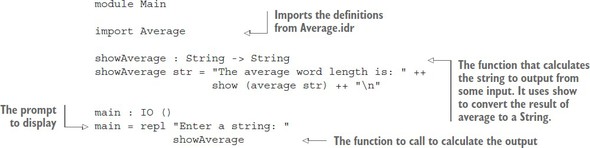
Again, you can use :exec to compile and run this at the REPL, and then try some inputs:
*AveMain> :exec Enter a string: The quick brown fox jumped over the lazy dog The average word length is: 4 Enter a string: The quick brown fox jumped over the lazy frog The average word length is: 4.11111 Enter a string:
Exercises
- What are the types of the following values?
- (“A”, “B”, “C”)
- [“A”, “B”, “C”]
- (('A', “B”), 'C')
- Write a palindrome function, of type String -> Bool, that returns whether the input reads the same backwards as forwards. Hint: You may find the function reverse : String -> String useful. You can test your answer at the REPL as follows:
*ex_2> palindrome "racecar" True : Bool *ex_2> palindrome "race car" False : Bool
- Modify the palindrome function so that it’s not case sensitive. Hint: You may find toLower : String -> String useful. You can test your answer at the REPL as follows:
*ex_2> palindrome "Racecar" True : Bool
- Modify the palindrome function so that it only returns True for strings longer than 10 characters. You can test your answer at the REPL as follows:
*ex_2> palindrome "racecar" False : Bool *ex_2> palindrome "able was i ere i saw elba" True : Bool
- Modify the palindrome function so that it only returns True for strings longer than some length given as an argument. Hint: Your new function should have type Nat -> String -> Bool. You can test your answer at the REPL as follows:
*ex_2> palindrome 10 "racecar" False : Bool *ex_2> palindrome 5 "racecar" True : Bool
- Write a counts function of type String -> (Nat, Nat) that returns a pair of the number of words in the input and the number of characters in the input. You can test your answer at the REPL as follows:
*ex_2> counts "Hello, Idris world!" (3, 19) : (Nat, Nat)
- Write a top_ten function of type Ord a => List a -> List a that returns the ten largest values in a list. You may find the following Prelude functions useful:
- take : Nat -> List a -> List a
- sort : Ord a => List a -> List a
*ex_2> top_ten [1..100] [100, 99, 98, 97, 96, 95, 94, 93, 92, 91] : List Integer
- Write an over_length function of type Nat -> List String -> Nat that returns the number of strings in the list longer than the given number of characters. You can test your answer at the REPL as follows:
*ex_2> over_length 3 ["One", "Two", "Three", "Four"] 2 : Nat
- For each of palindrome and counts, write a complete program that prompts for an input, calls the function, and prints its output. You can test your answer using :exec at the REPL:
*ex_2_palindrome> :exec Enter a string: Able was I ere I saw Elba True Enter a string: Madam, I'm Adam False Enter a string:
2.5. Summary
- The Prelude defines a number of basic types and functions and is imported automatically by all Idris programs.
- Idris provides basic numeric types, Int, Integer, Nat, and Double, as well as a Boolean type, Bool, a character type, Char, and a string type, String.
- Values can be converted between compatible types using the cast function, and can be given explicit types with the the function.
- Tuples are fixed-size collections where each element can be a different type.
- Lists are variable size collections where each element has the same type.
- Function types have one or more input types and one output type.
- Function types can be generic, meaning that they can contain variables. These variables can be constrained to allow a smaller set of types.
- Higher-order functions are functions in which one of the arguments is itself a function.
- Functions consist of a required type declaration and a definition. Function definitions are equations defining rewrite rules to be used during evaluation.
- Whitespace is significant in Idris programs. Each definition in a block must begin in exactly the same column.
- Function documentation can be accessed at the REPL with the :doc command.
- Idris programs can be divided into separate source files called modules.
- The entry point to an Idris program is the main function, which must have type IO (), and be defined in the module Main. Simple interactive programs can be written by applying the repl function from main.
Part 2. Core Idris
Now that you have some experience writing programs in Idris, it’s time to start your exploration of type-driven development in depth. In this part, you’ll learn about the core features of Idris and gain some experience in the process of type-driven development. Rather than showing you complete programs right from the start, I’ll show you how to build programs interactively, via a process of type, define, refine:
- Type— Write a type for a function.
- Define— Create an initial definition for the function, possibly containing holes.
- Refine— Complete the definition by filling in holes, possibly modifying the type as your understanding of the problem develops.
In chapter 3, you’ll learn the basics of interactive development; and then, in chapter 4, you’ll learn to define your own data types and build larger programs around them. Chapter 5 shows how you can write programs that interact with the outside world, using types to separate evaluation from execution. Later chapters introduce more-advanced concepts in type-driven development, including type-level computation in chapter 6, working with constrained generic types in chapter 7, describing and proving properties of programs in chapters 8 and 9, and defining alternative traversals of data structures using views in chapter 10.
By the end of part 2, you’ll have learned about all of the core features of Idris.
Chapter 3. Interactive development with types
This chapter covers
- Defining functions by pattern matching
- Type-driven interactive editing in Atom
- Adding precision to function types
- Practical programming with vectors
You’ve now seen how to define simple functions, and how to structure these into complete programs. In this chapter, we’ll start a deeper exploration into type-driven development. First, we’ll look at how to write more-complex functions with existing types from the Prelude, such as lists. Then, we’ll look at using the Idris type system to give functions more-precise types.
In type-driven development, we follow the process of “type, define, refine.” You’ll see this process in action throughout this chapter as you first write the types and, as far as possible, always have a type-correct, if perhaps incomplete, definition of a function and refine it step by step until it’s complete. Each step will be broadly characterized as one of these three:
- Type— Either write a type to begin the process, or inspect the type of a hole to decide how to continue the process.
- Define— Create the structure of a function definition either by creating an outline of a definition or breaking it down into smaller components.
- Refine— Improve an existing definition either by filling in a hole or making its type more precise.
In this chapter, I’ll introduce interactive development in the Atom text editor, which assists with this process. Atom provides an interactive editing mode that communicates with a running Idris system and uses types to help direct function development. Atom also provides some structural editing features and contextual information about functions with holes, and, when the types are precise enough, even completes large parts of functions for you. I’ll begin this chapter, therefore, by introducing the interactive editing mode in Atom.
Editor modes
Although we’ll use Atom to edit Idris programs, the interactive features we’ll use are provided by Idris itself. The Atom integration works by communicating with an Idris process running in the background. This process is run as a child of the editor, so it’s independent of any REPLs you may have running. As such, it’s reasonably straightforward to add Idris support to other text editors, and similar editing modes currently exist for Emacs and Vim. In this book, we’ll stick to Atom for consistency, but each of the commands directly maps to corresponding commands in other editors.
3.1. Interactive editing in Atom
You saw in chapter 1 that Idris programs can contain holes, which stand for parts of a function definition that haven’t yet been written. This is one way in which programs can be developed interactively: you write an incomplete definition containing holes, check the types of the holes to see what Idris expects in each, and then continue by filling in the holes with more code. There are several additional ways in which Idris can help you by integrating interactive development features with a text editor:
- Add definitions— Given a type declaration, Idris can add a skeleton definition of a function that satisfies that type.
- Case analysis— Given a skeleton function definition with arguments, Idris can use the types of those arguments to help define the function by pattern matching.
- Expression search— Given a hole with a precise enough type, Idris can try to find an expression that satisfies the hole’s type, refining the definition.
In this section, we’ll begin writing some more-complex Idris functions, using its interactive editing features to develop those functions, step by step, in a type-directed way. We’ll use the Atom text editor, because there’s an extension available for editing Idris programs, which can be installed directly from the default Atom distribution. The rest of this chapter assumes that you have the interactive Idris mode up and running. If not, follow the instructions in appendix A for installing Atom and the Idris mode.
3.1.1. Interactive command summary
Interactive editing in Atom involves a number of keyboard commands in the editor, which are summarized in table 3.1.Command mnemonics
For each command, the shortcut in Atom is to press Ctrl, Alt, and the first letter of the command.
Table 3.1. Interactive editing commands in Atom
| Shortcut | Command | Description |
|---|---|---|
| Ctrl-Alt-A | Add definition | Adds a skeleton definition for the name under the cursor |
| Ctrl-Alt-C | Case split | Splits a definition into pattern-matching clauses for the name under the cursor |
| Ctrl-Alt-D | Documentation | Displays documentation for the name under the cursor |
| Ctrl-Alt-L | Lift hole | Lifts a hole to the top level as a new function declaration |
| Ctrl-Alt-M | Match | Replaces a hole with a case expression that matches on an intermediate result |
| Ctrl-Alt-R | Reload | Reloads and type-checks the current buffer |
| Ctrl-Alt-S | Search | Searches for an expression that satisfies the type of the hole name under the cursor |
| Ctrl-Alt-T | Type-check name | Displays the type of the name under the cursor |
3.1.2. Defining functions by pattern matching
All of the function definitions we’ve looked at so far have involved a single equation to define that function’s behavior. For example, in the previous chapter you wrote a function to calculate the lengths of every word in a list:
allLengths : List String -> List Nat allLengths strs = map length strs
Here, you used functions defined in the Prelude (map and length) to inspect the list. At some stage, though, you’re going to need a more direct way to inspect values. After all, functions like map and length need to be defined themselves somehow!
In general, you define functions by pattern matching on the possible values of inputs to a function. For example, you can define a function to invert a Bool as follows:
invert : Bool -> Bool invert False = True invert True = False
The possible inputs of type Bool are True and False, so here you implement invert by listing the possible inputs and giving the corresponding outputs. Patterns can also contain variables, as illustrated by the following function, which returns "Empty" if given an empty list or "Non-empty" followed by the value of the tail if given a non-empty list:
describeList : List Int -> String describeList [] = "Empty" describeList (x :: xs) = "Non-empty, tail = " ++ show xs
Figure 3.1 illustrates how the patterns are matched in describeList for the inputs [1] (which is syntactic sugar for 1 :: []) and [2,3,4,5] (which is syntactic sugar for 2 :: 3 :: 4 :: 5 :: []).
Figure 3.1. Matching the pattern (x :: xs) for inputs [1] and [2,3,4,5]
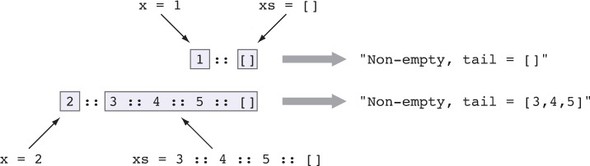
Naming conventions for lists
Conventionally, when working with lists and list-like structures, Idris programmers use a name ending in “s” (to suggest a plural), and then use its singular to refer to individual elements. So, if you have a list called things, you might refer to an element of the list as thing.
A function definition consists of one or more equations matching the possible inputs to that function. You can see how this works for lists if you implement allLengths by inspecting the list directly, instead of using map.
Listing 3.1. Calculating word lengths by pattern matching on the list (WordLength.idr)
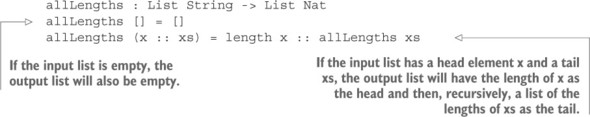
To see in detail how this definition is constructed, you’ll build it interactively in Atom. Each step can be broadly characterized as Type (creating or inspecting a type), Define (making a definition or breaking it down into separate clauses), or Refine (improving a definition by filling in a hole or making its type more precise).
- Type— First, start up Atom and create a WordLength.idr file containing the type declaration for allLengths. That’s only the following:
allLengths : List String -> List Nat
You should also start up an Idris REPL in a separate terminal so that you can type-check and test your definition:$ idris WordLength.idr ____ __ _ / _/___/ /____(_)____ / // __ / ___/ / ___/ Version 1.0 _/ // /_/ / / / (__ ) http://www.idris-lang.org/ /___/\__,_/_/ /_/____/ Type :? for help Idris is free software with ABSOLUTELY NO WARRANTY. For details type :warranty. Holes: Main.allLengths *WordLength>
- Define— In Atom, move the cursor over the name allLengths and press Ctrl-Alt-A. This will add a skeleton definition, and your editor buffer should now contain the following:
allLengths : List String -> List Nat allLengths xs = ?allLengths_rhs
The skeleton definition is always a clause with the appropriate number of arguments listed on the left side of the =, and with a hole on the right side. Idris uses various heuristics to choose initial names for the arguments. By convention, Idris chooses default names of xs, ys, or zs for Lists. - Type— You can check the types of holes in Atom by pressing Ctrl-Alt-T with the cursor over the hole you want to check. If you check the type of the allLengths_rhs hole, you should see this:
xs : List String -------------------------------------- allLengths_rhs : List Nat
- Define— You’ll write this definition by inspecting the list argument, named xs, directly. This means that for every form the list can take, you need to explain how to measure word lengths when it’s in that form. To tell the editor that you want to inspect the first argument, press Ctrl-Alt-C in Atom with the cursor over the variable xs in the first argument position. This expands the definition to give the two forms that the argument xs could take:
allLengths : List String -> List Nat allLengths [] = ?allLengths_rhs_1 allLengths (x :: xs) = ?allLengths_rhs_2
These are the two canonical forms of a list. That is, every list must be in one of these two forms: it can either be empty (in the form []), or it can be non-empty, containing a head element and the rest of the list (in the form (x :: xs)). It’s a good idea at this point to rename x and xs to something more meaningful than these default names:allLengths : List String -> List Nat allLengths [] = ?allLengths_rhs_1 allLengths (word :: words) = ?allLengths_rhs_2
In each case, there’s a new hole on the right side to fill in. You can check the types of these holes; type checking gives the expected return type and the types of any local variables. For example, if you check the type of allLengths_rhs_2, you’ll see the types of the local variables word and words, as well as the expected return type:word : String words : List String -------------------------------------- allLengths_rhs_2 : List Nat
- Refine— Idris has now told you which patterns are needed. Your job is to complete the definition by filling in the holes on the right side. In the case where the input is the empty list, the output is also the empty list, because there are no words for which to measure the length:
allLengths [] = []
- Refine— In the case where the input is non-empty, there’s a word as the first element (word) followed by the remainder of the list (words). You need to return a list with the length of word as its first element. For the moment, you can add a new hole (?rest) for the remainder of the list:
allLengths : List String -> List Nat allLengths [] = [] allLengths (word :: words) = length word :: ?rest
You can even test this incomplete definition at the REPL. Note that the REPL doesn’t reload files automatically, because it runs independently of the interactive editing in Atom, so you’ll need to reload explicitly using the :r command:*WordLength> :r Type Checking ./WordLength.idr Holes: Main.rest *WordLength> allLengths ["Hello", "Interactive", "Editors"] 5 :: ?rest : List Nat
For the hole rest, you need to calculate the lengths of the words in words. You can do this with a recursive call to allLengths, to complete the definition:allLengths : List String -> List Nat allLengths [] = [] allLengths (word :: words) = length word :: allLengths words
You now have a complete definition, which you can test at the REPL after reloading:
*WordLength> :r Type Checking ./WordLength.idr *WordLength> allLengths ["Hello", "Interactive", "Editors"] [5, 11, 7] : List Nat
It’s also a good idea to check whether Idris believes the definition is total.
*WordLength> :total allLengths Main.allLengths is Total
We’ll discuss totality checking in much more detail in chapters 10 and 11. For the moment, it’s sufficient to know that Idris will consider a function total if
- It has clauses that cover all possible well-typed inputs
- All recursive calls converge on a base case
As you’ll see in chapter 11 in particular, the definition of totality also allows interactive programs that run indefinitely, such as servers and interactive loops, provided they continue to produce intermediate results in finite time.
Idris believes that allLengths is total because there are clauses for all possible well-typed inputs, and the argument to the recursive call to allLengths is smaller (that is, closer to the base case) than the input.
3.1.3. Data types and patterns
When you press Ctrl-Alt-C in Atom with the cursor over a variable on the left side of a definition, it performs a case split on that variable, giving the possible patterns the variable can match. But where do these patterns come from?
Each data type has one or more constructors, which are the primitive ways of building values in that data type and give the patterns that can be matched for that data type. For List, there are two:
- Nil, which constructs an empty list
- ::, an infix operator that constructs a list from a head element and a tail
Additionally, as you saw in chapter 2, there’s syntactic sugar for lists that allows a list to be written as a comma-separated list of values in square brackets. Hence, Nil can also be written as [].
For any data type, you can find the constructors and thus the patterns to match using :doc at the REPL prompt:
Idris> :doc List Data type Prelude.List.List : (elem : Type) -> Type Generic lists Constructors: Nil : List elem Empty list (::) : (x : elem) -> (xs : List elem) -> List elem A non-empty list, consisting of a head element and the rest of the list. infixr 7
Documentation in Atom
You can get documentation directly in Atom by pressing Ctrl-Alt-D, with the cursor over the name for which you want documentation.
For Bool, for example, :doc reveals that the constructors are False and True:
Idris> :doc Bool Data type Prelude.Bool.Bool : Type Boolean Data Type Constructors: False : Bool True : Bool
Therefore, if you write a function that takes a Bool as an input, you can provide explicit cases for the inputs False and True.
For example, to write the exclusive OR operator, you could follow these steps:
- Type— Start by giving a type:
xor : Bool -> Bool -> Bool
- Define— Press Ctrl-Alt-A with the cursor over xor to add a skeleton definition:
xor : Bool -> Bool -> Bool xor x y = ?xor_rhs
- Define— Press Ctrl-Alt-C over the x to give the two possible cases for x:
xor : Bool -> Bool -> Bool xor False y = ?xor_rhs_1 xor True y = ?xor_rhs_2
- Refine— Complete the definition by filling in the right sides:
xor : Bool -> Bool -> Bool xor False y = y xor True y = not y
Type checking in Atom
While developing a function, and particularly when writing clauses by hand rather than using interactive editing features, it can be a good idea to type-check what you have so far. The Ctrl-Alt-R command rechecks the current buffer using the running Idris process. If it loads successfully, the Atom status bar will report “File loaded successfully.”
The Nat type, which represents unbounded unsigned integers, is also defined by primitive constructors. In Idris, a natural number is defined as being either zero, or one more than (that is, the successor of) another natural number.
Idris> :doc Nat Data type Prelude.Nat.Nat : Type Natural numbers: unbounded, unsigned integers which can be pattern matched. Constructors: Z : Nat Zero S : Nat -> Nat Successor
Data types and constructors
Data types are defined in terms of their constructors, as you’ll see in detail in chapter 4. The constructors of a data type are the primitive ways of building that data type, so in the case of Nat, every value of type Nat must be either zero or the successor of another Nat. The number 3, for example, is written in primitive form as S (S (S Z)). That is, it’s the successor (S) of 2 (written as S (S Z)).
Therefore, if you write a function that takes a Nat as an input, you can provide explicit cases for the number zero (Z) or a number greater than zero (S k, where k is any non-negative number). For example, to write an isEven function that returns True if a natural number input is divisible by 2, and returns False otherwise, you could define it recursively (if inefficiently) as follows:
- Type— Start by giving a type:
isEven : Nat -> Bool
- Define— Press Ctrl-Alt-A to add a skeleton definition:
isEven : Nat -> Bool isEven k = ?isEven_rhs
Naming conventions
As a naming convention, Idris chooses k by default for variables of type Nat. Naming conventions can be set by the programmer when defining data types, and you’ll see how to do this in chapter 4. In any case, it’s usually a good idea to rename these variables to something more informative.
- Define— Press Ctrl-Alt-C over the k to give the two possible cases for k:
isEven : Nat -> Bool isEven Z = ?isEven_rhs_1 isEven (S k) = ?isEven_rhs_2
To complete the definition, you have to explain what to return when the input is zero (Z) or when the input is non-zero (if the input takes the form S k, then k is a variable standing for a number that’s one smaller than the input). - Refine— Complete the definition by filling in the right sides:
isEven : Nat -> Bool isEven Z = True isEven (S k) = not (isEven k)
You’ve defined this recursively. Zero is an even number, so you return True for the input Z. If a number is even, its successor is odd, and vice versa, so you return not (isEven k) for the input S k.
It’s nevertheless sometimes useful to define two or more functions in terms of each other. This can be achieved in a mutual block. For example, you could define isEven in terms of an isOdd function, and vice versa:
mutual isEven : Nat -> Bool isEven Z = True isEven (S k) = isOdd k isOdd : Nat -> Bool isOdd Z = False isOdd (S k) = isEven k
3.2. Adding precision to types: working with vectors
In chapter 1, we discussed how having types as a first-class language construct allows us to define more-precise types. As one example, you saw how lists could be given more-precise types by including the number of elements in a list in its type, as well as the type of the elements. In Idris, a list that includes both the number and the type of elements in its type is called a vector, defined as the data type Vect. The following listing shows some example vectors.
Listing 3.2. Vectors: lists with lengths encoded in the type (Vectors.idr)
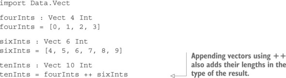
Vect isn’t defined in the Prelude, but it can be made available by importing the Data.Vect library module. Modules are imported with an import statement at the top of a source file:
import Data.Vect
Packages: prelude and base
Idris modules can be combined into packages, from which individual modules can be imported. The Prelude is defined in a package called prelude, from which all modules are imported automatically. Idris programs also have access to a package called base, which defines
several commonly useful data structures and algorithms including Vect, but from which modules must be imported explicitly. Up-to-date documentation for the packages distributed with Idris is available at www.idris-lang.org/documentation.3.2.1. Refining the type of allLengths
To see how Vect works, you can refine the type of the allLengths function from section 3.1.2 to use a Vect instead of a List, and redefine the function.
To do so, create a new source file called WordLength_vec.idr containing only the line import Data.Vect, and load it into the REPL. You can then check the documentation for Vect:
*WordLength_vec> :doc Vect Data type Data.Vect.Vect : Nat -> Type -> Type Vectors: Generic lists with explicit length in the type Constructors: Nil : Vect 0 a Empty vector (::) : (x : a) -> (xs : Vect k a) -> Vect (S k) a A non-empty vector of length S k, consisting of a head element and the rest of the list, of length k. infixr 7
Notice that it has the same constructors as List, but they have different types that give explicit lengths. Lengths are given as Nat, because they can’t be negative:
- The type of Nil explicitly states that the length is Z (displayed as the numeric literal 0 here).
- The type of :: explicitly states that the length is S k, given an element and a tail of length k.
The same syntactic sugar applies as for List, translating a bracketed list of values such as [1, 2, 3] to a sequence of :: and Nil: 1 :: 2 :: 3 :: Nil, in this case. In fact, this syntactic sugar applies to any data type with constructors called Nil and ::.
The constructor names for both List and Vect are the same, Nil and ::. Names can be overloaded, provided that different things with the same name are defined in separate namespaces, which in practice usually means separate modules. Idris will infer the appropriate namespace from the context in which the name is used.
You can explicitly indicate which of List or Vect is required using the:
Idris> the (List _) ["Hello", "There"] ["Hello", "There"] : List String Idris> the (Vect _ _) ["Hello", "There"] ["Hello", "There"] : Vect 2 StringThe underscore (_) in the preceding expressions indicates to Idris that you would like it to infer a value for that argument. You can use _ in an expression whenever there’s only one valid value that would stand for that expression. You’ll see more about this in section 3.4.
To define allLengths using a Vect, you can follow a similar procedure as when defining it using List. The difference is that you must consider how the lengths of the input and output are related.
Figure 3.2 shows how, in the output list, there’s always an entry corresponding to an entry in the input list. Therefore, you can make it explicit in the type that the output vector has the same length as the input vector:
allLengths : Vect len String -> Vect len Nat
Figure 3.2. Calculating the lengths of words in a list. Notice that each input has a corresponding output, so the length of the output vector is always the same as the length of the input vector.
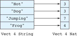
The len that appears in the input is a variable at the type level, standing for the length of the input. Because the output uses the same variable at the type level, it’s explicit in the type that the output has the same length as the input. Here’s how you can write the function:
- Type— Create an Atom buffer with the following contents to import Data.Vect and give the type of allLengths:
import Data.Vect allLengths : Vect len String -> Vect len Nat
- Define— As before, create a skeleton definition with Ctrl-Alt-A:
allLengths : Vect len String -> Vect len Nat allLengths xs = ?allLengths_rhs
- Define— As before, press Ctrl-Alt-C over the xs to tell Idris that you’d like to define the function by pattern matching on xs:
allLengths : Vect len String -> Vect len Nat allLengths [] = ?allLengths_rhs_1 allLengths (x :: xs) = ?allLengths_rhs_2
As before, it’s a good idea at this point to rename the variables x and xs to something more meaningful:allLengths : Vect len String -> Vect len Nat allLengths [] = ?allLengths_rhs_1 allLengths (word :: words) = ?allLengths_rhs_2
- Type— If you now inspect the types of the holes allLengths_rhs_1 and allLengths_rhs_2, you’ll see more information than in the List version, because the types are more precise. For example, in allLengths_rhs_1 you can see that the only valid result is a vector with zero elements:
-------------------------------------- allLengths_rhs_1 : Vect 0 Nat
In allLengths_rhs_2 you can see how the lengths of the pattern variables and output relate to each other, given some natural number n:word : String k : Nat words : Vect k String -------------------------------------- allLengths_rhs_2 : Vect (S k) Nat
That is, in the pattern (word :: words), word is a String, words is a vector of kStrings, and for the output you need to provide a vector of Nat of length 1 + k, represented as S k. - Refine— For allLengths_rhs_1, there’s only one vector that has length zero, which is the empty vector, so there’s only one value you can use to refine the definition by filling in the hole:
allLengths : Vect len String -> Vect len Nat allLengths [] = [] allLengths (word :: words) = ?allLengths_rhs_2
- Refine— For allLengths_rhs_2, the required type is Vect (S k) Nat, so the result must be a non-empty vector (using ::). Also, you can make a value of type Vect k Nat by calling allLengths recursively. You can leave a hole for the first element in the resulting list, refining the definition by hand as follows:
allLengths : Vect len String -> Vect len Nat allLengths [] = [] allLengths (word :: words) = ?wordlen :: allLengths words
You still have one hole in this result, ?wordlen, which will be the length of the first word:word : String k : Nat words : Vect k String -------------------------------------- wordlen : Nat
- Refine— To complete the definition, fill in the remaining hole by calculating the length of the word x:
allLengths : Vect len String -> Vect len Nat allLengths [] = [] allLengths (word :: words) = length word :: allLengths words
The more precise type, describing how the lengths of the input and output relate, means that the interactive editing mode can tell you more about the expressions you’re looking for. You can also be more confident that the program behaves as intended by ruling out any program that doesn’t preserve length by type-checking.
Nat and data structures
You might notice a direct correspondence between the constructors of Vect and the constructors of Nat. When you add an element to a Vect with ::, you add an S constructor to its length. In practice, capturing the size of data structures like this is a very common use of Nat.
To illustrate how the more precise type rules out some incorrect programs, consider the following implementation of allLengths, using List instead of Vect:
allLengths : List String -> List Nat allLengths xs = []
This is well typed and it will be accepted by Idris, but it won’t work as intended because there’s no guarantee that the output list has an entry corresponding to each entry in the input. On the other hand, the following program with the more precise type is not well typed and will not be accepted by Idris:
allLengths : Vect n String -> Vect n Nat allLengths xs = []
This results in the following type error, which states that an empty vector was given when a vector of length n was needed:
WordLength_vec.idr:4:14:When checking right hand side of allLengths: Type mismatch between Vect 0 Nat (Type of []) and Vect n Nat (Expected type)
As with the previous List-based version of allLengths, you can check that your new definition is total at the REPL:
*WordLength_vec> :total allLengths Main.allLengths is Total
If, for example, you remove the case for the empty list, you have a definition that is well typed but partial:
allLengths : Vect len String -> Vect len Nat allLengths (word :: words) = length word :: allLengths words
When you check this for totality, you’ll see this:
*WordLength_vec> :total allLengths Main.allLengths is not total as there are missing cases
total allLengths : Vect len String -> Vect len Nat allLengths [] = [] allLengths (word :: words) = length word :: allLengths words
The total keyword before the type declaration means that Idris will report an error if the definition isn’t total. For example, if you remove the allLengths [] case, this is what Idris will report:
WordLength_vec.idr:5:1: Main.allLengths is not total as there are missing cases
3.2.2. Type-directed search: automatic refining
After step 3 in the previous section, you had the patterns for allLengths and holes for the right sides, which you provided by refining directly:
allLengths : Vect n String -> Vect n Nat allLengths [] = ?allLengths_rhs_1 allLengths (word :: words) = ?allLengths_rhs_2
Take another look at the types and the local variables for the allLengths_rhs_1 and allLengths_rhs_2 holes:
-------------------------------------- allLengths_rhs_1 : Vect 0 Nat word : String k : Nat words : Vect k String -------------------------------------- allLengths_rhs_2 : Vect (S k) Nat
By looking carefully at the types, you could see how to construct values to fill these holes. But not only do you have more information here, so does Idris!
Given enough information in the type, Idris can search for a valid expression that satisfies the type. In Atom, press Ctrl-Alt-S over the allLengths_rhs_1 hole, and you should see that the definition has changed:
allLengths : Vect n String -> Vect n Nat allLengths [] = [] allLengths (word :: words) = ?allLengths_rhs_2
Because there’s only one possible value for a vector of length zero, Idris has refined this automatically.
You can also try an expression search on the allLengths_rhs_2 hole. Press Ctrl-Alt-S with the cursor over allLengths_rhs_2, and you should see this:
allLengths : Vect n String -> Vect n Nat allLengths [] = [] allLengths (word :: words) = 0 :: allLengths wordsThe required type was Vect (S k) Nat so, as before, Idris realized that the only possible result would be a non-empty vector. It also realized that it could find a value of type Vect k Nat by calling allLengths recursively on words.
For the Nat at the head of the vector, Idris has found the first value that satisfies the type, 0, but this isn’t exactly what you want, so you can replace it with a hole—?vecthead:
allLengths : Vect n String -> Vect n Nat allLengths [] = [] allLengths (word :: words) = ?vecthead :: allLengths words
Checking the type of ?vecthead confirms that you’re looking for a Nat:
word : String k : Nat words : Vect k String -------------------------------------- vecthead : Nat
As before, you can complete the definition by filling this hole with length word. So, not only does the more precise type give you more confidence in the correctness of the program and give you more information when writing the program, it also gives Idris some information, allowing it to write a good bit of the program for you.
3.2.3. Type, define, refine: sorting a vector
For all the functions you’ve written so far in this chapter, you’ve followed this process:
- Write a type.
- Create a skeleton definition.
- Pattern match on an argument.
- Fill in the holes on the right side with a combination of type-driven expression search and refining holes by hand.
Usually, there’s a little more work to do, however. For example, you may find you need to create additional helper functions, inspect intermediate results, or refine the type you initially gave for a function.
You can see this in practice by creating a function that returns a sorted version of an input vector. You can use insertion sort, which is a simple sorting algorithm that’s easily implemented in a functional style, informally described as follows:
- Given an empty vector, return an empty vector.
- Given the head and tail of a vector, sort the tail of the vector and then insert the head into the sorted tail such that the result remains sorted.
You can write this interactively, beginning with the skeleton definition shown in listing 3.3. Open an Atom buffer and put this code into a file called VecSort.idr. Remember that you can create the skeleton definition of insSort from the type with Ctrl-Alt-A.
Listing 3.3. A skeleton definition of insSort on vectors with an initial type (VecSort.idr)
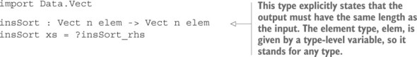
As you work through this process, I recommend that you inspect the types of each of the holes that arise using Ctrl-Alt-T, and ensure that you understand the types of the variables and the holes.
Development workflow
It’s typically useful to have an Atom window open for interactively editing a file, as well as a terminal window with a REPL open for testing, evaluation, checking documentation, and so on.
Having written the type for this function, implement it by doing the following:
- Define— Case-split on xs with Ctrl-Alt-C, leading to this:
insSort : Vect n elem -> Vect n elem insSort [] = ?insSort_rhs_1 insSort (x :: xs) = ?insSort_rhs_2
- Refine— Try an expression search on ?insSort_rhs_1, leading to this:
insSort : Vect n elem -> Vect n elem insSort [] = [] insSort (x :: xs) = ?insSort_rhs_2
A sorted empty vector is itself an empty vector, as expected. - Refine— Trying an expression search on ?insSort_rhs_2 is, unfortunately, less effective:
insSort : Vect n elem -> Vect n elem insSort [] = [] insSort (x :: xs) = x :: xs
Although Idris knows how long the vector should be, and it has local variables of the correct types, the overall type of insSort isn’t precise enough for Idris to fill in the hole with the program you intend.Expression search
As this example demonstrates, although expression search can often lead you to a valid function, it’s not a substitute for understanding how the program works! You need to understand the algorithm, but you can use expression search to help fill in the details.
- Define— When you’re writing a function over a recursive data type, it’s often effective to make recursive calls to the recursive parts of the structure. Here, you can sort the tail with a recursive call to insSort xs and bind the result to a locally defined variable:
insSort : Vect n elem -> Vect n elem insSort [] = [] insSort (x :: xs) = let xsSorted = insSort xs in ?insSort_rhs_2
- Type— In ?insSort_rhs_2 you’re going to insert the head x into the sorted tail, xsSorted. Because this is going to be a little more complex, you can lift the hole to a top-level definition by pressing Ctrl-Alt-L with the cursor over ?-insSort_rhs_2, which leads to the following:
insSort_rhs_2 : (x : elem) -> (xs : Vect k elem) -> (xsSorted : Vect k elem) -> Vect (S k) elem insSort : Vect n elem -> Vect n elem insSort [] = [] insSort (x :: xs) = let xsSorted = insSort xs in insSort_rhs_2 x xs xsSorted
This has created a new top-level function with a new type but no implementation, and it has replaced the hole with a call to the new function. The arguments to the new function are the local variables that were in scope in the hole ?insSort_rhs_2. - Refine— Once you realize that the job of the new function is to insert x into the xsSorted vector, you can edit the name and type of insSort_rhs_2 to reflect this. You can remove the arguments that you aren’t going to need:
insert : (x : elem) -> (xsSorted : Vect k elem) -> Vect (S k) elem insSort : Vect n elem -> Vect n elem insSort [] = [] insSort (x :: xs) = let xsSorted = insSort xs in insert x xsSorted
Lifting Definitions
When lifting a definition with Ctrl-Alt-L, Idris will generate a new definition with the same name as the hole, using all of the local variables in the generated type. In this case, you know you aren’t going to need all of them, so you can edit out the unnecessary xs argument.
- Define— You now have to define insert. Again, create a skeleton definition:
insert : (x : elem) -> (xsSorted : Vect k elem) -> Vect (S k) elem insert x xsSorted = ?insert_rhs
Then case-split on xsSorted, leading to this:insert : (x : elem) -> (xsSorted : Vect k elem) -> Vect (S k) elem insert x [] = ?insert_rhs_1 insert x (y :: xs) = ?insert_rhs_2
- Refine— An expression search on insert_rhs_1 leads to the following:
insert : (x : elem) -> (xsSorted : Vect k elem) -> Vect (S k) elem insert x [] = [x] insert x (y :: xs) = ?insert_rhs_2
This works because Idris knows it’s looking for a vector with one element of type elem, and the only thing available with type elem is x. - Refine— For the (y :: xs) case, with the hole ?insert_rhs_2, you have a problem. There are two cases to consider:
- If x < y, the result should be x :: y :: xs, because the result won’t be ordered if x is inserted after y.
- Otherwise, the result should begin with y, and then have x inserted into the tail xs.
insert : Ord elem => (x : elem) -> (xsSorted : Vect k elem) -> Vect (S k) elem insert x [] = [x] insert x (y :: xs) = ?insert_rhs_2 insSort : Ord elem => Vect n elem -> Vect n elem insSort [] = [] insSort (x :: xs) = let xsSorted = insSort xs in insert x xsSorted
Remember from chapter 2 that you constrain generic types by placing constraints such as Ord elem before => in the type. You’ll see more about this in chapter 7. - Define— You now need to check x < y and act on the result. One way to do this is with an if...then...else construct:
insert : Ord elem => (x : elem) -> (xsSorted : Vect k elem) -> Vect (S k) elem insert x [] = [x] insert x (y :: xs) = if x < y then x :: y :: xs else y :: insert x xs
Alternatively, you can use interactive editing to give more structure to the definition, and insert a case construct to match on an intermediate result. Press Ctrl-Alt-M with the cursor over ?insert_rhs_2. This introduces a new case expression with a placeholder for the value to be inspected (so the function won’t type-check yet):insert : Ord elem => (x : elem) -> (xsSorted : Vect k elem) -> Vect (S k) elem insert x [] = [x] insert x (y :: xs) = case _ of case_val => ?insert_rhs_2
The _ stands for an expression you need to provide in order for the function to type-check successfully. You’ll need to fill in the _ with the expression you want to match:insert : Ord elem => (x : elem) -> (xsSorted : Vect k elem) -> Vect (S k) elem insert x [] = [x] insert x (y :: xs) = case x < y of case_val => ?insert_rhs_2
- Define— You can now case-split on case_val in the usual way, with Ctrl-Alt-C, leading to this:
insert : Ord elem => (x : elem) -> (xsSorted : Vect k elem) -> Vect (S k) elem insert x [] = [x] insert x (y :: xs) = case x < y of False => ?insert_rhs_1 True => ?insert_rhs_3
- Refine— Finally, you complete the implementation by filling in the new holes insert_rhs_1 and insert_rhs_3. Unfortunately, expression search won’t help you much here because there’s not enough information in the type, so you need to fill these in by hand:
insert : Ord elem => (x : elem) -> (xsSorted : Vect k elem) -> Vect (S k) elem insert x [] = [x] insert x (y :: xs) = case x < y of False => y :: insert x xs True => x :: y :: xs
Once the definition is complete, you can test it at the REPL, like this:
*VecSort> insSort [1,3,2,9,7,6,4,5,8] [1, 2, 3, 4, 5, 6, 7, 8, 9] : Vect 9 Integer
Don’t forget to check that insSort is total:
*VecSort> :total insSort Main.insSort is Total
It’s a good habit to check that the functions you define are total. If a function is type-correct, but not total, it might appear to work when you test it, but there might still be a subtle error on some unusual inputs, such as a missing pattern or possible nontermination.
- Written a type for insSort.
- Tried to define insSort until you encountered the need to insert, which you lifted to a new top-level definition with its own type.
- Tried to define insert until you encountered the need to compare, at which point you refined the types to support the ordering constraint on elem.
- Continued to define insert using the refined type, and hence completed the implementation of insSort.
Exercises
To conclude this section, here are some exercises to test your understanding of the interactive editing mode and pattern matching on List and Vect.
The following functions, or some variant on them, are defined in the Prelude or in Data.Vect:
- length : List a -> Nat
- reverse : List a -> List a
- map : (a -> b) -> List a -> List b
- map : (a -> b) -> Vect n a -> Vect n b
For each of them, define your own version using interactive editing in Atom. Note that you’ll need to use different names (such as my_length, my_reverse, my_map) to avoid clashing with the names in the Prelude. You can test your answers at the REPL as follows:
*ex_3_2> my_length [1..10] 10 : Nat *ex_3_2> my_reverse [1..10] [10, 9, 8, 7, 6, 5, 4, 3, 2, 1] : List Integer *ex_3_2> my_map (* 2) [1..10] [2, 4, 6, 8, 10, 12, 14, 16, 18, 20] : List Integer *ex_3_2> my_vect_map length ["Hot", "Dog", "Jumping", "Frog"] [3, 3, 7, 4] : Vect 4 Nat
Don’t forget to check that your definitions are total!
3.3. Example: type-driven development of matrix functions
The main reason you might use vectors, with the length explicit in the type, as opposed to lists, is to have the lengths of the vectors help guide you to a working function more quickly. This can be particularly helpful when you work with two-dimensional vectors. These, in turn, can be helpful for implementing operations on matrices, which have several applications in programming, such as 3D graphics.
A matrix, in mathematics, is a rectangular array of numbers arranged in rows and columns. Figure 3.3 shows an example 3 × 4 matrix in both mathematical notation,
and in Idris notation as a vector of vectors. Notice that when representing a matrix as nested vectors, the dimensions of the matrix become explicit in the type.Figure 3.3. Representation of a matrix as two-dimensional vectors. On the left, the matrix is in mathematical notation. The same matrix is represented in Idris on the right.
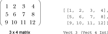
3.3.1. Matrix operations and their types
When implementing operations on matrices, such as addition and multiplication, it’s important to check that the dimensions of the vectors you’re working with are appropriate for the operations. For example:
- When adding matrices, each matrix must have exactly the same dimensions. Addition works by adding corresponding elements in each matrix. For example, you can add two 3 × 2 matrices as follows:
The following addition of a 2 × 2 matrix to a 3 × 2 matrix is invalid because there are no corresponding elements in the third row: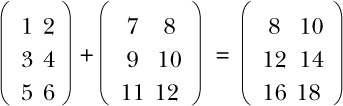
So, the type of matrix addition could be as follows: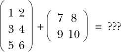
addMatrix : Num numType => Vect rows (Vect cols numType) -> Vect rows (Vect cols numType) -> Vect rows (Vect cols numType)
In other words, for some numeric type numType, adding a rows × cols matrix to a rows × cols matrix results in a rows × cols matrix. - When multiplying matrices, the number of columns in the left matrix must be the same as the number of rows in the right matrix. Then, multiplication works as follows:
Here, multiplying a 3 × 2 matrix by a 2 × 4 matrix results in a 3 × 4 matrix. The value in row x, column y in the result is the sum of the product of corresponding elements in row x of the left input, and column y of the right input. So the type of matrix multiplication could be as follows: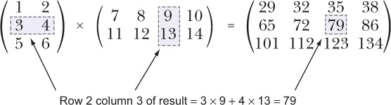
multMatrix : Num numType => Vect n (Vect m numType) -> Vect m (Vect p numType) -> Vect n (Vect p numType)
In other words, for some numeric type numType, multiplying an n × m matrix by an m × p matrix results in an n × p matrix.
3.3.2. Transposing a matrix
A useful operation when manipulating matrices is transposition, which converts rows to columns and vice versa. For example, a 3 × 2 matrix becomes a 2 × 3 matrix:
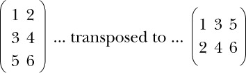
You can write a transposeMat function that, in general, converts an m × n matrix into an n × m matrix, representing matrices as nested vectors. As usual, you can write the function interactively, where each step is broadly characterized as one of type, define, or refine. From this point, I’ll generally assume you’re comfortable with the interactive commands in Atom, and I’ll describe the overall type-driven process rather than the specifics of building the function.
- Type— Begin by giving a type for transposeMat:
transposeMat : Vect m (Vect n elem) -> Vect n (Vect m elem)
For matrix arithmetic, in the types of addMatrix and multMatrix, you need to constrain the element type to be numeric. Here, though, the element type of the matrix, elem, could be anything. You’re not going to inspect it or use it at any point in the implementation of transposeMat; you merely change the rows to columns and columns to rows. - Define— Create a skeleton definition, and then case-split on the input vector:
transposeMat : Vect m (Vect n elem) -> Vect n (Vect m elem) transposeMat [] = ?transposeMat_rhs_1 transposeMat (x :: xs) = ?transposeMat_rhs_2
- Type— When Idris creates new holes, either from a case split or an incomplete result of an expression search, it’s always a good idea to inspect the types of those holes to get some insight into how to proceed. First, take a look at the type of ?transposeMat_rhs_1:
elem : Type n : Nat -------------------------------------- transposeMat_rhs_1 : Vect n (Vect 0 elem)
Here, you’re trying to convert a 0 × n vector into an n × 0 vector, so you need to create n copies of an empty vector. We’ll return to this case later; for now, you can rename the hole to createEmpties and lift it to a top-level function with Ctrl-Alt-L:createEmpties : Vect n (Vect 0 elem) transposeMat : Vect m (Vect n elem) -> Vect n (Vect m elem) transposeMat [] = createEmpties transposeMat (x :: xs) = ?transposeMat_rhs_2
- Type— Look at the type of ?transposeMat_rhs_2:
elem : Type n : Nat x : Vect n elem k : Nat xs : Vect k (Vect n elem) -------------------------------------- transposeMat_rhs_2 : Vect n (Vect (S k) elem)
You have xs, which is a k × n matrix, and you need to make an n × (S k) matrix. - Define— One insight you need here is that it’s likely easier to build an n × (S k) matrix from an n × k matrix, because at least one of the dimensions is correct. You can create such a matrix by transposing xs:
transposeMat (x :: xs) = let xsTrans = transposeMat xs in ?transposeMat_rhs_2
- Type— You can also lift ?transposeMat_rhs_2 to a top-level function, renaming it transposeHelper. This results in the following:
transposeHelper : (x : Vect n elem) -> (xs : Vect k (Vect n elem)) -> (xsTrans : Vect n (Vect k elem)) -> Vect n (Vect (S k) elem)
The type for transposeHelper is generated from the types of the local variables you have access to: x, xs, and xsTrans. It will take these variables as inputs, and produce a Vect n (Vect (S k) elem) as output. - Type— At this stage, it’s good to look more closely at the types of the variables x, xs, and xsTrans and try to use these types to visualize what you need to do to complete transposeMat. For the sake of visualization, let’s take n = 4 and k = 2. Figure 3.4 shows an original two-dimensional vector, of the form (x :: xs), where x is the first row and xs is the rest of the rows, built with these dimensions. It identifies the components x and xs, and it shows the result of transposing xs and the expected result of the whole operation.
Figure 3.4. The components of the vector you’re transposing (x and xs), along with the result of transposing xs, and the expected overall result
What you need to do, therefore, is add each element of x to the vector in the corresponding element of xsTrans; you won’t need xs in transposeHelper. If you delete this by hand in the type of transposeHelper and the application in transposeMat, you get this: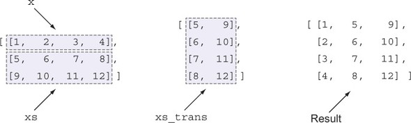
transposeHelper : (x : Vect n elem) -> (xsTrans : Vect n (Vect k elem)) -> Vect n (Vect (S k) elem) transposeMat : Vect m (Vect n elem) -> Vect n (Vect m elem) transposeMat [] = createEmpties transposeMat (x :: xs) = let xsTrans = transposeMat xs in transposeHelper x xsTrans
- Define— To implement transposeHelper, you can add a skeleton definition, pattern match on x and xsTrans, and then use expression search to complete the definition. There’s enough information for Idris to fill in the details itself:
transposeHelper : (x : Vect n elem) -> (xsTrans : Vect n (Vect k elem)) -> Vect n (Vect (S k) elem) transposeHelper [] [] = [] transposeHelper (x :: xs) (y :: ys) = (x :: y) :: transposeHelper xs ys
Rather than typing this in directly, try to build it using the interactive commands. It’s possible to write this function from the type using only Ctrl-Alt-A, Ctrl-Alt-C, Ctrl-Alt-S, and cursor movements.Case splitting on vectors
If you case-split on x and then case-split on xsTrans, notice that Idris only gives one possible pattern for xsTrans. This is because the types of x and xsTrans state that both must have the same length.
- Define— All that remains is to implement createEmpties. You can implement this using a library function, replicate:
*transpose> :doc Vect.replicate Data.Vect.replicate : (n : Nat) -> (x : a) -> Vect n a Repeat some value n times Arguments: n : Nat -- the number of times to repeat it x : a -- the value to repeat
If you create a skeleton definition of createEmpties from its type, you’ll see the following:createEmpties : Vect n (Vect 0 elem) createEmpties = ?createEmpties_rhs
You need to call replicate to build a vector of n empty lists. Unfortunately, because there are no local variables available from the patterns on the left side, the natural definition results in an error message:createEmpties : Vect n (Vect 0 elem) createEmpties = replicate n [] -- "No such variable n"
The problem is that n is a type-level variable, and not accessible to the definition of createEmpties. Shortly, in section 3.4, you’ll see how to handle type-level variables in general, and how you might write createEmpties directly. For the moment, because the type dictates that there’s only one valid value for the length argument to replicate, you can use an underscore instead:createEmpties : Vect n (Vect 0 elem) createEmpties = replicate _ []
The implementation of transposeMat is now complete. For reference, the complete definition is given in listing 3.4. You can test it at the REPL:
*transpose> transposeMat [[1,2], [3,4], [5,6]] [[1, 3, 5], [2, 4, 6]] : Vect 2 (Vect 3 Integer)
Listing 3.4. Complete definition of matrix transposition (Matrix.idr)
createEmpties : Vect n (Vect 0 elem) createEmpties = replicate _ [] transposeHelper : (x : Vect n elem) -> (xsTrans : Vect n (Vect k elem)) -> Vect n (Vect (S k) elem) transposeHelper [] [] = [] transposeHelper (x :: xs) (y :: ys) = (x :: y) :: transposeHelper xs ys transposeMat : Vect m (Vect n elem) -> Vect n (Vect m elem) transposeMat [] = createEmpties transposeMat (x :: xs) = let xsTrans = transposeMat xs in transposeHelper x xsTrans
When building a definition interactively using the type-define-refine process, it’s good to look out for parts of the definition that could be made more generic, or that could instead be implemented using existing library functions.
For example, transposeHelper has a structure very similar to the library function zipWith, which applies a function to corresponding elements in two vectors and is defined as follows:
zipWith : (a -> b -> c) -> Vect n a -> Vect n b -> Vect n c zipWith f [] [] = [] zipWith f (x :: xs) (y :: ys) = f x y :: zipWith f xs ys
Exercises
- Reimplement transposeMat using zipWith instead of transposeHelper. You can test your answer at the REPL as follows:
*ex_3_3_3> transposeMat [[1,2], [3,4], [5,6]] [[1, 3, 5], [2, 4, 6]] : Vect 2 (Vect 3 Integer)
- Implement addMatrix : Num a => Vect n (Vect m a) -> Vect n (Vect m a) -> Vect n (Vect m a). You can test your answer at the REPL as follows:
*ex_3_3_3> addMatrix [[1,2], [3,4]] [[5,6], [7,8]] [[6, 8], [10, 12]] : Vect 2 (Vect 2 Integer)
- Implement a function for multiplying matrices, following the description given in section 3.3.1. Hint: This definition is quite tricky and involves multiple steps. Consider the following:
- You have a left matrix of dimensions n × m, and a right matrix of dimensions m × p. A good start is to use transposeMat on the right matrix.
- Remember that you can use Ctrl-Alt-L to lift holes to top-level functions.
- Remember to pay close attention to the types of the local variables and the types of the holes.
- Remember to use Ctrl-Alt-S to search for expressions, and pay close attention to the types of any resulting holes.
*ex_3_3_3> multMatrix [[1,2], [3,4], [5,6]] [[7,8,9,10], [11,12,13,14]] [[29, 32, 35, 38], [65, 72, 79, 86], [101, 112, 123, 134]] : Vect 3 (Vect 4 Integer)
3.4. Implicit arguments: type-level variables
You’ve now seen several definitions with variables at the type level that can stand either for types or values. For example:reverse : List elem -> List elem
Here, elem is a type-level variable standing for the element type of the list. It appears twice, in the input type and the return type, so the element type of each must be the same.
append : Vect n elem -> Vect m elem -> Vect (n + m) elem
Here, elem is again a type-level variable standing for the element type of the vectors. n and m are type-level variables standing for the lengths of the input vectors, and they’re used again in the output to describe how the length of the output relates to the length of the inputs.
These type-level variables aren’t declared anywhere else. Because types are first class, type-level variables can also be brought into scope and used in definitions. These type-level variables are referred to as implicit arguments to the functions reverse and append. In this section, you’ll see how implicit arguments work, and how to use them in definitions.
3.4.1. The need for implicit arguments
To illustrate the need for implicit arguments, let’s take a look at how you might define append without them. You could make the elem, n, and m arguments to append explicit, resulting in the following definition:
append : (elem : Type) -> (n : Nat) -> (m : Nat) -> Vect n elem -> Vect m elem -> Vect (n + m) elem append elem Z m [] ys = ys append elem (S k) m (x :: xs) ys = x :: append elem k m xs ys
But if you did so, you’d also have to be explicit about the element type and lengths when calling append:
*Append_expl> append Char 2 2 ['a','b'] ['c','d'] ['a', 'b', 'c', 'd'] : Vect 4 Char
Given the types of the arguments ['a', 'b'] and ['c', 'd'], there’s only one possible value for each of the arguments elem (which must be a Char), n (which must be 2, from the length of ['a', 'b']), and m (which must also be 2, from the length of ['c','d']). Any other value for any of these would not be well typed.
Because there is enough information in the types of the vector arguments, Idris can infer the values for the a, n, and m arguments. You can therefore write this:
*Append> append _ _ _ ['a','b'] ['c','d'] ['a', 'b', 'c', 'd'] : Vect 4 Char
*Append> append _ _ _ ['a','b'] ['c','d'] ['a', 'b', 'c', 'd'] : Vect 4 Char
Idris will report an error if it can’t:
*Append> append _ _ _ _ ['c','d'] (input):Can't infer argument n to append, Can't infer explicit argument to append
Here, Idris reports that it can’t work out the length of the first vector, or the first vector itself. Unlike holes, which stand for parts of expressions that aren’t yet written, underscores stand for parts of expressions for which there’s only one valid value. It’s an error if Idris can’t infer a unique value for an underscore.
Using implicit arguments avoids the need for writing details explicitly that can be inferred by Idris. Making elem, n, and m implicit in the type of append means that you can refer to them directly in the type where necessary, without needing to give explicit values when calling the function.
3.4.2. Bound and unbound implicits
Let’s take another look at the types of reverse and append, with implicit arguments:
reverse : List elem -> List elem append : Vect n elem -> Vect m elem -> Vect (n + m) elem
The names elem, n, and m are called unbound implicits. This is because their names are used directly, without being declared (or bound) anywhere else. You could also have written these types as follows:
reverse : {elem : Type} -> List elem -> List elem append : {elem : Type} -> {n : Nat} -> {m : Nat} -> Vect n elem -> Vect m elem -> Vect (n + m) elem Here, the implicit arguments have been explicitly bound in the type. The notation {x : S} -> T denotes a function type where the argument is intended to be inferred by Idris, rather than written directly by the programmer.
When you write a type with unbound implicits, Idris will look for undefined names in the type, and turn them internally into bound implicits. Consider this example:
append : Vect n elem -> Vect m elem -> Vect (n + m) elem
First, Idris identifies that elem, n, and m are undefined, so it internally rewrites the type as follows:
append : {elem : _} -> {n : _} -> {m : _} -> Vect n elem -> Vect m elem -> Vect (n + m) elem Note that it has not attempted to fill in types for the new arguments, but instead has given them as underscores in the hope that it will be able to infer them from some other information in the rest of the type. Here, this results in the following: append : {elem : Type} -> {n : Nat} -> {m : Nat} -> Vect n elem -> Vect m elem -> Vect (n + m) elem In practice, Idris will not treat every undefined name as an unbound implicit—only names that begin with a lowercase letter and that appear either on their own or in a function argument position. Given the following,
test : f m a -> b -> a
m appears in an argument position, as does a. b appears on its own, and f only appears in a function position. As a result, m, a, and b are treated as unbound implicits. f isn’t treated as an unbound implicit, meaning that it must be defined elsewhere for this type to be valid.
Normally, for conciseness, you leave implicits unbound, but in some situations, it’s useful to use bound implicits instead:
- For clarity and readability, it can be useful to give explicit types to implicit arguments.
- If there’s a dependency between an implicit argument and some other argument, you may need to use a bound implicit to make this clear to Idris.
3.4.3. Using implicit arguments in functions
Internally, Idris treats implicit arguments like any other argument, but with the notational convenience that the programmer doesn’t need to provide them explicitly. As a result, you can refer to implicit arguments inside function definitions, and even case-split on them.
For example, how can you find the length of a vector? You could do this by case splitting on the vector itself:
length : Vect n elem -> Nat length [] = Z length (x :: xs) = 1 + length xs
Because the length is part of the type, you could also refer to it directly:
length : Vect n elem -> Nat length {n} xs = n The notation {n} in a pattern brings the implicit argument n into scope, allowing you to use it directly.
More generally, you can give explicit values for implicit arguments by using the notation {n = value}, where n is the name of an implicit argument:
*Append> append {elem = Char} {n = 2} {m = 3} append : Vect 2 Char -> Vect 3 Char -> Vect 5 Char Here, you’ve partially applied append to its implicit arguments only, giving a specialized function for appending a vector of two Chars to a vector of three Chars.
This notation can also be used on the left side of a definition to case-split on an implicit argument. For example, to implement createEmpties in section 3.3.2, you could have written it directly by case splitting on the length n after bringing it into scope:
createEmpties : Vect n (Vect 0 a) createEmpties {n} = ?createEmpties_rhs If you case-split on n in Atom, you’ll see this:
createEmpties : Vect n (Vect 0 a) createEmpties {n = Z} = ?createEmpties_rhs_1 createEmpties {n = (S k)} = ?createEmpties_rhs_2 Finally, you can complete the definition with an expression search for both of the remaining holes:
createEmpties : Vect n (Vect 0 a) createEmpties {n = Z} = [] createEmpties {n = (S k)} = [] :: createEmpties Note that in the recursive call, createEmpties is sufficient. There’s no need to provide an explicit value for the length because only one value (k) would type-check. On the other hand, if you try at the REPL without a value for the length, Idris will report an error:
*transpose> createEmpties (input):Can't infer argument n to createEmpties, Can't infer argument a to createEmpties
You can solve this either by giving explicit values for n and elem, or giving a target type for the expression:
*transpose> createEmpties {a=Int} {n=4} [[], [], [], []] : Vect 4 (Vect 0 Int) *transpose> the (Vect 4 (Vect 0 Int)) createEmpties [[], [], [], []] : Vect 4 (Vect 0 Int) Because implicit arguments are, internally, treated the same as any other argument, you might wonder what happens at runtime. Generally, you use implicit arguments to give precise types to programs, so does this mean that type information has to be compiled and present at runtime?
Fortunately, the Idris compiler is aware of this problem. It will analyze a program before compiling it so that any arguments that are only used for type checking won’t be present at runtime.
3.5. Summary
- Functions in Idris are defined by collections of pattern-matching equations.
- Patterns arise from the constructors of a data type.
- The Atom text editor provides an interactive editing mode that uses the type to help direct function implementation. Similar modes are available for Emacs and Vim.
- Interactive editing commands provide natural tools for following the process of type, define, refine.
- Interactive editing provides a command for searching for a valid expression that satisfies the type of a hole.
- More-precise types, such as Vect, give more information to the compiler both to help check that a function is correct, and to help constrain expression searches.
- Matrices are two-dimensional vectors, with the dimensions encoded in the type. Operations on matrices such as addition and multiplication can be given types that precisely describe how the operations affect the dimensions.
- The type-define-refine process helps you to implement matrix operations with precise types by using the type to direct the implementation of each subexpression and create appropriate helper functions.
- Type-level variables are implicit arguments to functions, which can be brought into scope and used like any other arguments by enclosing them in braces {}.
Chapter 4. User-defined data types
This chapter covers
- Defining your own data types
- Understanding different forms of data types
- Writing larger interactive programs in the type-driven style
Type-driven development involves not only giving precise types to functions, as you’ve seen so far, but also thinking about exactly how data is structured. In a sense, programming (pure functional programming, in particular) is about transforming data from one form to another. Types allow us to describe the form of that data, and the more precise we make these descriptions, the more guidance the language can give in implementing transformations on that data.
Several useful data types are distributed as part of the Idris libraries, many of which we’ve used so far, such as List, Bool, and Vect. Other than being defined directly in Idris, there’s nothing special about these data types. In any realistic program, you’ll need to define your own data types to capture the specific requirements of the problem you’re solving and the specific forms of data you’re working with. Not only that, but there’s a significant payoff to thinking carefully about the design of data types: the more precisely types capture the requirements of a problem, the more benefit you’ll get from interactive type-directed editing.
In this chapter, therefore, we’ll look at how to define new data types. You’ll see the various forms of data types in a number of small example functions. We’ll also start to work on a larger example, an interactive data store, that we’ll extend in the coming chapters. At first, we’ll store only strings, accessing them by an integer index, but even in this small example you’ll see how user-defined types and dependent types can help build an interactive interface, dealing safely with possible runtime errors.4.1. Defining data types
Data types are defined by a type constructor and one or more data constructors. In fact, you’ve already seen these when you used :doc to see the details of a data type. For example, the following listing shows the output of :doc List, annotated to highlight the type and data constructors.
Listing 4.1. Type and data constructors from :doc
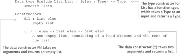
Using data constructors is the canonical way of building the types given by the type constructor. In the case of List, this means that every value with a type of the form List elem is either Nil or takes the form x :: xs for some element x and the remainder of the list, xs.
We’ll classify types into five basic groups, although they’re all defined with the same syntax:
- Enumerated types— Types defined by giving the possible values directly
- Union types— Enumerated types that carry additional data with each value
- Recursive types— Union types that are defined in terms of themselves
- Generic types— Types that are parameterized over some other types
- Dependent types— Types that are computed from some other value
In this section, you’ll see how to define enumerated types, union types, recursive types, and generic types; we’ll discuss dependent types in the next section. If you’ve programmed in a functional language before, or in any language that allows you to define generic types, the types we discuss in this section should be familiar, even if the notation is new.
Naming conventions
By convention, I’ll use an initial capital letter for both type constructors and data constructors, and an initial lowercase letter for functions. There’s no requirement to do so, but it gives a useful visual indication to the reader of the code.4.1.1. Enumerations
An enumerated type is directly defined by giving the valid values for that type. The simplest example is Bool, which is defined as follows in the Prelude:
data Bool = False | True
To define an enumerated data type, you give the data keyword to introduce the declaration, and then give the name of the type constructor (in this case, Bool) and list the names of the data constructors (in this case True and False).
Figure 4.1 shows another example, defining an enumerated type for representing the four cardinal points on a compass.
Figure 4.1. Defining a Direction data type (Direction.idr)
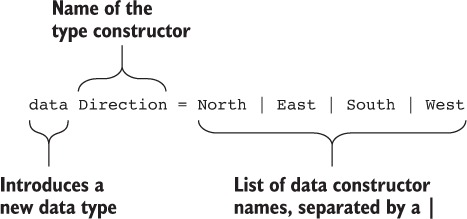
Data constructor names are separated by a vertical bar, |, and there’s no restriction on how the declaration is laid out (other than the usual layout rule that all declarations begin in precisely the same column). For example, they could each be on a different line:
data Direction = North | East | South | West
Once you’ve defined a data type, you can use it to define functions interactively. For example, you could define a turnClockwise function as follows, with the usual process of type, define, refine:
- Type— Write a function type with Direction as the input and output, and then create a skeleton definition:
turnClockwise : Direction -> Direction turnClockwise x = ?turnClockwise_rhs
- Define— Define the function by case splitting on x:
turnClockwise : Direction -> Direction turnClockwise North = ?turnClockwise_rhs_1 turnClockwise East = ?turnClockwise_rhs_2 turnClockwise South = ?turnClockwise_rhs_3 turnClockwise West = ?turnClockwise_rhs_4
- Refine— Fill in the holes on the right sides:
turnClockwise : Direction -> Direction turnClockwise North = East turnClockwise East = South turnClockwise South = West turnClockwise West = North
4.1.2. Union types
A union type is an extension of an enumerated type in which the constructors of the type can themselves carry data. For example, you could create an enumeration type for shapes:
data Shape = Triangle | Rectangle | Circle
You may want to store more information with a shape, so that you can draw it, for example, or calculate its area. This information will differ depending on the shape:
- For a triangle, you might want to know the length of its base and its height.
- For a rectangle, you might want to know its length and height.
- For a circle, you might want to know its radius.
To represent this information, each of the data constructors, Triangle, Rectangle, and Circle, can be given argument types that carry this data using Doubles to represent dimensions. Figure 4.2 shows some example shapes and their representations.
Figure 4.2. Example shapes represented as a union type. Triangle takes two Doubles, for base and height; Rectangle takes two Doubles, for width and height; Circle takes a Double for radius.
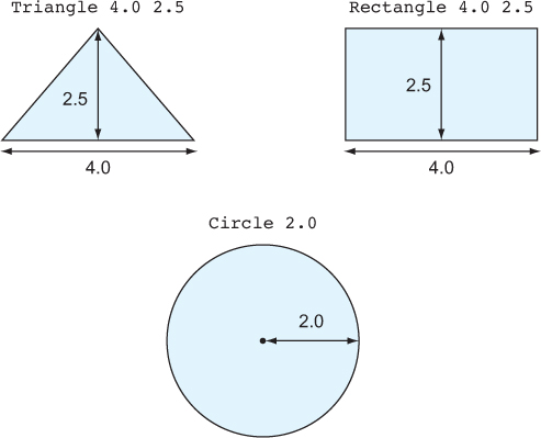
You can represent shapes in this form as an Idris data type:
data Shape = Triangle Double Double | Rectangle Double Double | Circle Double
Listing 4.2 shows how you might define an area function that calculates the area of a shape for each of these possibilities. As an exercise, rather than typing in this function directly, try to construct it using the interactive editing tools in Atom.
Listing 4.2. Defining a Shape type and calculating its area (Shape.idr)
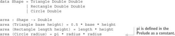
If you check the documentation for Shape using :doc, you can see how this data declaration translates into type and data constructors:
*Shape> :doc Shape Data type Main.Shape : Type Constructors: Triangle : Double -> Double -> Shape Rectangle : Double -> Double -> Shape Circle : Double -> Shape
When you define new data types, it’s also a good idea to provide documentation that will be displayed with :doc, using documentation comments. In this case, it helps indicate what each Double is for. Documentation comments are laid out in data declarations by giving the comment before each constructor:
||| Represents shapes data Shape = ||| A triangle, with its base length and height Triangle Double Double | ||| A rectangle, with its length and height Rectangle Double Double | ||| A circle, with its radius Circle Double
This is rendered as follows with :doc:
*Shape> :doc Shape Data type Main.Shape : Type Represents shapes Constructors: Triangle : Double -> Double -> Shape A triangle, with its base length and height Rectangle : Double -> Double -> Shape A rectangle, with its length and height Circle : Double -> Shape A circle, with its radius
data Shape = Triangle Double Double | Rectangle Double Double | Circle Double
It’s also possible to define data types by giving their type and data constructors directly, in the form shown by :doc. You could define Shape as follows:
data Shape : Type where Triangle : Double -> Double -> Shape Rectangle : Double -> Double -> Shape Circle : Double -> Shape
This is identical to the previous declaration. In this case, it’s a little more verbose, but this syntax is more general and flexible. You’ll see more of this shortly when we define dependent types.
I’ll use both syntaxes throughout the book. Generally, I’ll use the concise form, unless I need the additional flexibility.
4.1.3. Recursive types
Types can also be recursive, that is, defined in terms of themselves. For example, Nat is defined recursively in the Prelude as follows:
data Nat = Z | S Nat
The Prelude also defines functions and notation to allow Nat to be used like any other numeric type, so rather than writing S (S (S (S Z))), you can simply write 4. Nevertheless, in its primitive form it’s defined using data constructors.
It would be reasonable to be concerned about the efficiency of Nat given that it’s defined in terms of constructors. There’s no need to worry, though, for three reasons:
- In practice, Nat is primarily used structurally, to describe the size of a data structure such as Vect in its type, so the size of a Nat corresponds to the size of the data structure itself.
- When a program is compiled, types are erased, so a Nat that appears at the type level, such as in the length of a Vect, is erased.
- Internally, the compiler optimizes the representation of Nat so that it’s really stored as a machine integer.
You can use a recursive type to extend the Shape example from the previous section to represent larger pictures. We’ll define a picture as being one of the following:
- A primitive shape
- A combination of two other pictures
- A picture rotated through an angle
- A picture translated to a different location
Note that three of these are defined in terms of pictures themselves. You could define a picture type following the preceding informal description, as shown next.
Listing 4.3. Defining a Picture type recursively, consisting of Shapes and smaller Pictures (Picture.idr)
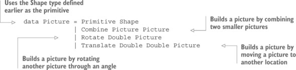
Figure 4.3 shows an example of the sort of picture you could represent with this data type. For each of the primitive shapes, we’ll consider its location to be the top left of an imaginary box that bounds the shape.
Figure 4.3. An example picture combining three shapes translated to different positions
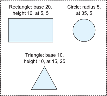
We know that there are three subpictures, so to represent this in code, you can begin (define) by using Combine to put three subpictures together:
testPicture : Picture testPicture = Combine ?pic1 (Combine ?pic2 ?pic3)
To continue, you know that each subpicture is translated to a specific position, so you can fill in those details (refine), leaving holes for the primitive shapes themselves:
testPicture : Picture testPicture = Combine (Translate 5 5 ?rectangle) (Combine (Translate 35 5 ?circle) (Translate 15 25 ?triangle))
Finally, you can fill in (refine) the details of the individual primitive shapes. One way to do this is to use Ctrl-Alt-L in Atom to lift the holes to the top level (type), and then fill in the definition, resulting in the following final definition.
Listing 4.4. The picture from figure 4.3 represented in code (Picture.idr)
As usual, you write functions over the Picture data type by case splitting. To write a function that calculates the area of every primitive shape in a picture, you can begin by writing a type:
pictureArea : Picture -> Double
Then, create a skeleton definition and case-split on its argument. You should reach the following:
pictureArea : Picture -> Double pictureArea (Primitive x) = ?pictureArea_rhs_1 pictureArea (Combine x y) = ?pictureArea_rhs_2 pictureArea (Rotate x y) = ?pictureArea_rhs_3 pictureArea (Translate x y z) = ?pictureArea_rhs_4
This has given you an outline definition, showing you the forms the input can take and giving holes on the right side.
The names of the variables x, y, and z, chosen by Idris when creating the patterns for pictureArea, are not particularly informative. You can tell Idris how to choose better default names using the %name directive:
%name Shape shape, shape1, shape2 %name Picture pic, pic1, pic2
Now, when Idris needs to choose a variable name for a variable of type Shape, it will choose shape by default, followed by shape1 if shape is already in scope, followed by shape2. Similarly, it will choose pic, pic1, or pic2 for variables of type Picture.
After adding %name directives, case splitting on the argument will lead to patterns with more-informative variable names:pictureArea : Picture -> Double pictureArea (Primitive shape) = ?pictureArea_rhs_1 pictureArea (Combine pic pic1) = ?pictureArea_rhs_2 pictureArea (Rotate x pic) = ?pictureArea_rhs_3 pictureArea (Translate x y pic) = ?pictureArea_rhs_4
The completed definition is given in listing 4.5. For every Picture you encounter in the structure, you recursively call pictureArea, and when you encounter a Shape, you call the area function defined previously.
Listing 4.5. Calculating the total area of all shapes in a Picture (Picture.idr)
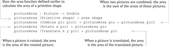
It’s always a good idea to test the resulting definition at the REPL:
*Picture> pictureArea testPicture 328.5398163397473 : Double
Recursive data types, just like recursive functions, need at least one non-recursive case in order to be useful, so at least one of the constructors needs to have a non-recursive argument. If you don’t do this, you’ll never be able to construct an element of that type. For example:
data Infinite = Forever Infinite
It is, however, possible to work with infinite streams of data using a generic Inf type, which we’ll explore in chapter 11.
4.1.4. Generic data types
A generic data type is a type that’s parameterized over some other type. Just like generic function types, which you saw in chapter 2, generic data types allow you to capture common patterns of data.
To illustrate the need for generic data types, consider a function that returns the area of the largest triangle in a Picture, as defined in the previous section. At first, you might write the following type:
biggestTriangle : Picture -> Double
But what should it return if there are no triangles in the picture? You could return some kind of sentinel value, like a negative size, but this would be against the spirit of type-driven development because you’d be using Double to represent something that isn’t really a number. Idris also doesn’t have a null value. Instead, you could refine the type of biggestTriangle, introducing a new union type for capturing the possibility that there are no triangles:
data Biggest = NoTriangle | Size Double biggestTriangle : Picture -> Biggest
I’ll leave the definition of biggestTriangle as an exercise.
You might also want to write a type that represents the possibility of failure. For example, you could write a safe division function for Double that returns an error if dividing by zero:
data DivResult = DivByZero | Result Double safeDivide : Double -> Double -> DivResult safeDivide x y = if y == 0 then DivByZero else Result (x / y)
Both Biggest and DivResult have the same structure! Instead of defining multiple types of this form, you can define one single generic type. In fact, such a generic type exists in the Prelude, called Maybe. The following listing shows the definition of Maybe.
Listing 4.6. A generic type, Maybe, that captures the possibility of failure
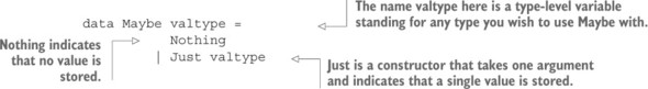
In a generic type, we use type variables such as valtype here to stand for concrete types. You can now define safeDivide using Maybe Double instead of DivResult, instantiating valtype with Double:
safeDivide : Double -> Double -> Maybe Double safeDivide x y = if y == 0 then Nothing else Just (x / y)
We’ve already written several functions with a generic type, List, which is defined in the Prelude as follows:
data List elem = Nil | (::) elem (List elem)
Generic data types can have more than one parameter, as illustrated in figure 4.4 for Either, which is defined in the Prelude and represents a choice between two alternative types.
Figure 4.4. Defining the Either data type
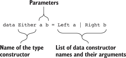
You might hear people informally referring to “the List type” or “the Maybe type.” It’s not strictly accurate to do this, however. List on its own is not a type, as you can confirm at the REPL:
Idris> :t List List : Type -> Type
Technically, List has a function type that takes a Type as a parameter and returns a Type. Although List Int is a type because it has been applied to a concrete argument, List itself is not. Instead, we’ll informally refer to List as a generic type.
One useful example of a generic type is a binary tree structure. The following listing shows the definition of binary trees, using a %name directive to give naming hints for building definitions interactively.
Listing 4.7. Defining binary trees (Tree.idr)
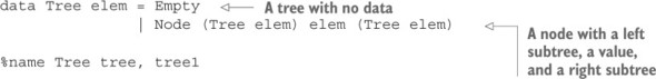
Binary trees are commonly used to store ordered information, where everything in a node’s left subtree is smaller than the value at the node, and everything in a node’s right subtree is larger than the value at the node.
Such trees are called binary search trees, and you can write a function to insert a value into such a tree, provided that you can order those values:
insert : Ord elem => elem -> Tree elem -> Tree elem insert x tree = ?insert_rhs
To write this function, create a Tree.idr file containing the definition in listing 4.7, and do the following:
- Define— Case-split on the tree, giving the cases where the tree is Empty and where the tree is a Node:
insert : Ord elem => elem -> Tree elem -> Tree elem insert x Empty = ?insert_rhs_1 insert x (Node tree y tree1) = ?insert_rhs_2
Even with the %name directive, the names tree, y, and tree1 aren’t especially informative, so let’s rename them to indicate that they’re the left subtree, the value at the node, and the right subtree, respectively:insert : Ord elem => elem -> Tree elem -> Tree elem insert x Empty = ?insert_rhs_1 insert x (Node left val right) = ?insert_rhs_2
- Refine— For ?insert_rhs_1, you create a new tree node with empty subtrees:
insert : Ord elem => elem -> Tree elem -> Tree elem insert x Empty = Node Empty x Empty insert x (Node left val right) = ?insert_rhs_2
- Define— For ?insert_rhs_2, you need to compare the value you’re inserting, x, with the value at the node, val. If x is smaller than val, you insert it into the left subtree. If it’s equal, it’s already in the tree, so you return the tree unchanged. If it’s greater than val, you insert it into the right subtree. To do this, you can use the compare function from the Prelude, which returns an element of an Ordering enumeration:
data Ordering = LT | EQ | GT compare : Ord a => a -> a -> Ordering
You’ll perform a match on the intermediate result of compare x val. Press Ctrl-Alt-M over insert_rhs_2:insert : Ord elem => elem -> Tree elem -> Tree elem insert x Empty = Node Empty x Empty insert x (Node left val right) = case _ of case_val => ?insert_rhs_2
- Define— The case expression won’t type-check until the _ is replaced with an expression to test, so replace it with compare x val:
insert : Ord elem => elem -> Tree elem -> Tree elem insert x Empty = Node Empty x Empty insert x (Node left val right) = case compare x val of case_val => ?insert_rhs_2
- Define— If you now case-split on case_val, you’ll get the patterns for LT, EQ, and GT:
insert : Ord elem => elem -> Tree elem -> Tree elem insert x Empty = Node Empty x Empty insert x (Node left val right) = case compare x val of LT => ?insert_rhs_1 EQ => ?insert_rhs_3 GT => ?insert_rhs_4
The following listing shows the complete definition of this function, after refining the remaining holes.
Listing 4.8. Inserting a value into a binary search tree (Tree.idr)
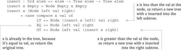
In insert, you might have noticed that in the EQ branch, the value you returned was exactly the same as the pattern on the left side. As a notational convenience, you can also name patterns:
insert x orig@(Node left val right) = case compare x val of LT => Node (insert x left) val right EQ => orig GT => Node left val (insert x right)
The notation orig@(Node left val right) gives the name orig to the pattern Node left val right. It doesn’t change the meaning of the pattern match, but it does mean that you can use the name orig on the right side rather than repeating the pattern.
There needs to be an Ord constraint on the generic variable elem in the type of insert, because otherwise you wouldn’t be able to use compare. An alternative approach would be to capture the Ord constraint in the tree type itself, refining the type to include this extra precision. The following listing shows how to do this by giving the type and data constructors directly.
Listing 4.9. A binary search tree with the ordering constraint in the type (BSTree.idr)
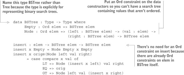
Precision and reuse
Putting a constraint in the tree structure itself makes the type more precise, in that it can now only store values that can be compared at the nodes, but at the cost of making it less reusable. This is a trade-off you’ll often have to consider when defining new data types. There are various ways of managing this trade-off, such as pairing data with predicates that describe the form of that data, as you’ll see in chapter 9.
Exercises
- Write a function, listToTree : Ord a => List a -> Tree a, that inserts every element of a list into a binary search tree. You can test this at the REPL as follows:
*ex_4_1> listToTree [1,4,3,5,2] Node (Node Empty 1 Empty) 2 (Node (Node Empty 3 (Node Empty 4 Empty)) 5 Empty) : Tree Integer
- Write a corresponding function, treeToList : Tree a -> List a, that flattens a tree into a list using in-order traversal (that is, all the values in the left subtree of a node should be added to the list before the value at the node, which should be added before the values in the right subtree). If you have the correct answers to exercises 1 and 2, you should be able to run this:
*ex_4_1> treeToList (listToTree [4,1,8,7,2,3,9,5,6]) [1, 2, 3, 4, 5, 6, 7, 8, 9] : List Integer
- An integer arithmetic expression can take one of the following forms:
- A single integer
- Addition of an expression to an expression
- Subtraction of an expression from an expression
- Multiplication of an expression with an expression
- Write a function, evaluate : Expr -> Int, that evaluates an integer arithmetic expression. If you have correct answers to 3 and 4, you should be able to try something like the following at the REPL:
*ex_4_1> evaluate (Mult (Val 10) (Add (Val 6) (Val 3))) 90 : Int
- Write a function, maxMaybe : Ord a => Maybe a -> Maybe a -> Maybe a, that returns the larger of the two inputs, or Nothing if both inputs are Nothing. For example:
*ex_4_1> maxMaybe (Just 4) (Just 5) Just 5 : Maybe Integer *ex_4_1> maxMaybe (Just 4) Nothing Just 4 : Maybe Integer
- Write a function, biggestTriangle : Picture -> Maybe Double, that returns the area of the biggest triangle in a picture, or Nothing if there are no triangles. For example, you can define the following pictures:
testPic1 : Picture testPic1 = Combine (Primitive (Triangle 2 3)) (Primitive (Triangle 2 4)) testPic2 : Picture testPic2 = Combine (Primitive (Rectangle 1 3)) (Primitive (Circle 4))
Then, test biggestTriangle at the REPL as follows:*ex_4_1> biggestTriangle testPic1 Just 4.0 : Maybe Double *ex_4_1> biggestTriangle testPic2 Nothing : Maybe Double
4.2. Defining dependent data types
A dependent data type is a type that’s computed from some other value. You’ve already seen a dependent type, Vect, where the exact type is calculated from the vector’s length:Vect : Nat -> Type -> Type
In other words, the type of a Vect depends on its length. This gives us additional precision in the type, which we used to help direct our programming via the process of type, define, refine. In this section, you’ll see how to define dependent types such as Vect. The core of the idea is that, because there’s no syntactic distinction between types and expressions, types can be computed from any expression.
We’ll begin with a simple example to illustrate how this works, defining a type for representing vehicles and their properties, depending on their power source, and you’ll see how you can use this to constrain the valid inputs to a function to those that make sense. You’ll then see how Vect itself is defined, along with some useful operations on it.
4.2.1. A first example: classifying vehicles by power source
Dependent types allow you to give more precise information about the data constructors of a type, by adding more arguments to the type constructor. For example, you might have a data type to represent vehicles (for example, bicycles, cars, and buses), but some operations don’t make sense on all values in the type (for example, refueling a bicycle wouldn’t work because there’s no fuel tank). We’ll therefore classify vehicles into those powered by pedal and those powered by petrol, and express this in the type.
The following listing shows how you could express this in Idris.
Listing 4.10. Defining a dependent type for vehicles, with their power source in the type (vehicle.idr)

You can write functions that will work on all vehicles by using a type variable to stand for the power source. For example, all vehicles have a number of wheels. On the other hand, not all vehicles carry fuel, so it only makes sense to refuel a vehicle whose type indicates it’s powered by Petrol. Both of these concepts are illustrated in the following listing.
Listing 4.11. Reading and updating properties of Vehicle
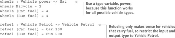
If you try adding a case for refueling a Bicycle, Idris will report a type error, because the input type is restricted to vehicles powered by petrol. If you use the interactive tools, Idris won’t even give a case for Bicycle after a case split with Ctrl-Alt-C. Nevertheless, it can sometimes aid readability to make it explicit that you know the Bicycle case is impossible. You can write this:
refuel : Vehicle Petrol -> Vehicle Petrol refuel (Car fuel) = Car 100 refuel (Bus fuel) = Bus 200 refuel Bicycle impossible
If you do this, Idris will check that the case you have marked as impossible would produce a type error.
Similarly, if you assert a case is impossible but Idris believes it’s valid, it will report an error:
refuel : Vehicle Petrol -> Vehicle Petrol refuel (Car fuel) = Car 100 refuel (Bus fuel) impossible
Here, Idris will report the following:
vehicle.idr:15:8:refuel (Bus fuel) is a valid case
In general, you should define dependent types by giving the type constructor and the data constructors directly. This gives you a lot of flexibility in the form that the constructors can take. Here, it has allowed you to define types where the data constructors can each take different arguments. You can either write functions that work on all vehicles (like wheels) or functions that only work on some subset of vehicles (like refuel).
Defining families of types
For Vehicle, you’ve actually defined two types in one declaration (specifically, Vehicle Pedal and Vehicle Petrol). Dependent data types like Vehicle are therefore sometimes referred to as families of types, because you’re defining multiple related types at the same time. The power source is an index of the Vehicle family. The index tells you exactly which Vehicle type you mean.
4.2.2. Defining vectors
In chapter 3, we looked at the ways we could use the length information in the type to help drive development of functions on vectors. In this section, we’ll look at how Vect is defined, along with some of the operations on it.It’s defined in the Data.Vect module, as shown in listing 4.12. The type constructor, Vect, takes a length and an element type as arguments, so when you define the data constructors, you state explicitly in their types what their lengths are.
Listing 4.12. Defining vectors (Vect.idr)
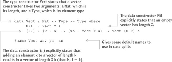
The Data.Vect library includes several utility functions on Vect, including concatenation, looking up values by their position in the vector, and various higher-order functions, such as map. Instead of importing this, though, we’ll use our own definition of Vect and try writing some functions by hand. To begin, create a Vect.idr file containing only the definition of Vect in listing 4.12.
Because Vect includes the length explicitly in its type, any function that uses some instance of Vect will describe its length properties explicitly in its type. For example, if you define an append function on Vect, its type will express how the lengths of the inputs and output are related:
append : Vect n elem -> Vect m elem -> Vect (n + m) elem
Type-level expressions
The expression n + m in the return type here is an ordinary expression with type Nat, using the ordinary + operator. Because Vect’s first argument is of type Nat, you should expect to be able to use any expression of type Nat. Remember, types are first-class, so types and expressions are all part of the same language.
Having written the type first, as always, you can define append by case splitting on the first argument. You do this interactively as follows:
- Define— Begin by creating a skeleton definition and then case splitting on the first argument xs:
append : Vect n elem -> Vect m elem -> Vect (n + m) elem append [] ys = ?append_rhs_1 append (x :: xs) ys = ?append_rhs_2
- Refine— Idris has enough information in the type to complete this definition by an expression search on each of the holes, resulting in this:
append : Vect n elem -> Vect m elem -> Vect (n + m) elem append [] ys = ys append (x :: xs) ys = x :: append xs ys
Vect defines a family of types, and we say that a Vect is indexed by its length and parameterized by an element type. The distinction between parameters and indices is as follows:
- A parameter is unchanged across the entire structure. In this case, every element of the vector has the same type.
- An index may change across a structure. In this case, every subvector has a different length.
The distinction is most useful when looking at a function’s type: you can be certain that the specific value of a parameter can play no part in a function’s definition. The index, however, might, as you’ve already seen in chapter 3 when defining length for vectors by looking at the length index, and when defining createEmpties for building a vector of empty vectors.
Another common operation on vectors is zip, which pairs corresponding elements in two vectors, as illustrated in figure 4.5.
Figure 4.5. Pairing corresponding elements of [1,2,3,4] and ["one","two","three","four"] using zip
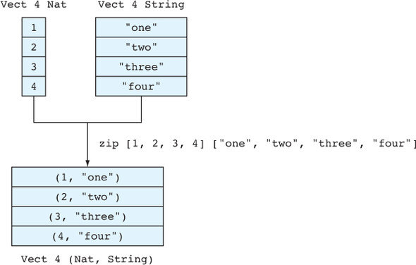
The name zip is intended to suggest the workings of a zip fastener, bringing two sides of a bag or jacket together. Because the length of each input Vect is in the type, you need to think about how the lengths of the inputs and output will correspond. A reasonable choice for this would be to require the lengths of both inputs to be the same:
zip : Vect n a -> Vect n b -> Vect n (a, b)
Having a more precise type for Vect, capturing the length in the type, means that you need to decide in advance how the lengths of the inputs to zip relate and express this decision in the type. Also, it means you can safely assume that zip will only ever be called with equal length lists, because if this assumption is violated, Idris will report a type error.
You can define zip, as usual, step by step:
- Define— Again, you can begin to define this by a case split on the first argument:
zip : Vect n a -> Vect n b -> Vect n (a, b) zip [] ys = ?zip_rhs_1 zip (x :: xs) ys = ?zip_rhs_2
- Refine— You can fill in ?zip_rhs_1 with an expression search, because the only well-typed result is an empty vector:
zip : Vect n a -> Vect n b -> Vect n (a, b) zip [] ys = [] zip (x :: xs) ys = ?zip_rhs_2
- Refine— For the second case, ?zip_rhs_2, take a look at the type of the hole and see if that gives you further information about what to do:
b : Type a : Type x : a k : Nat xs : Vect k a ys : Vect (S k) b -------------------------------------- zip_rhs_2 : Vect (S k) (a, b)
Notice that ys has length S k, meaning that there must be at least one element. If you case-split on ys, Idris won’t give you a pattern for the empty list, because it wouldn’t be a well-typed value:zip : Vect n a -> Vect n b -> Vect n (a, b) zip [] ys = [] zip (x :: xs) (y :: ys) = ?zip_rhs_1
After the case split, Idris has created a new hole, so let’s take a look at the types of the local variables:b : Type a : Type x : a k : Nat xs : Vect k a y : b ys : Vect k b -------------------------------------- zip_rhs_1 : Vect (S k) (a, b)
Again, there’s enough information to complete the definition with an expression search:zip : Vect n a -> Vect n b -> Vect n (a, b) zip [] ys = [] zip (x :: xs) (y :: ys) = (x, y) :: zip xs ys
Idris has noticed that it needs to build a vector of length S k, that it can create the appropriate vector of length k with a recursive call, and that it can create the appropriate first element by pairing x and y.
To understand what expression search has done, it can be instructive to remove some part of the result and replace it with a hole, to see what type expression search was working with at that point. For example, you can remove the (x, y):
zip : Vect n a -> Vect n b -> Vect n (a, b) zip [] ys = [] zip (x :: xs) (y :: ys) = ?element :: zip xs ys
Then, checking the type of the ?element hole, you’ll see that at this point, Idris was looking for a pair of a and b:
b : Type a : Type x : a k : Nat xs : Vect k a y : b ys : Vect k b -------------------------------------- element : (a, b)
The only way to make a pair of a and b at this point is to use x and y, so this is what Idris used to construct the pair.
4.2.3. Indexing vectors with bounded numbers using Fin
Because Vects carry their length as part of their type, the type checker has additional knowledge that it can use to check that operations are implemented and used correctly. One example is that if you wish to look up an element in a Vect by its location in the vector, you can know at compile time that the location can’t be out of bounds when the program is run.
The index function, defined in Data.Vect, is a bounds-safe lookup function whose type guarantees that it will never access a location that’s outside the bounds of a vector:
index : Fin n -> Vect n a -> a
The first argument, of type Fin n, is an unsigned number that has a non-inclusive upper bound of n. The name Fin suggests that the number is finitely bounded. So, for example, when you look up an element by location, you can use a number within the bounds of the vector:
Idris> :module Data.Vect *Data/Vect> Vect.index 3 [1,2,3,4,5]
Importing modules at the REPL
In the element lookup example, you import Data.Vect at the REPL using the :module command, to get access to the index function. There are several functions in the Prelude called index for indexing different list-like structures, so you have to disambiguate explicitly with Vect.index here.
But if you try to use a number outside the bounds, you’ll get a type error:
*Data/Vect> Vect.index 7 [1,2,3,4,5] (input):1:14:When checking argument prf to function Data.Fin.fromInteger: When using 7 as a literal for a Fin 5 7 is not strictly less than 5
Integer literal notation
As with Nat, you can use integer literals for Fin, provided that the compiler can be sure that the literal is within the bounds stated in the type.
If you’re reading a number as user input that will be used to index a Vect, the number won’t always be within the bounds of the Vect. In practice, you’ll often need to convert from an arbitrarily sized Integer to a bounded Fin.
Importing Data.Vect gives you access to the integerToFin function, which converts an Integer to a Fin with some bounds, provided the Integer is within bounds. It has the following type:
integerToFin : Integer -> (n : Nat) -> Maybe (Fin n)
The first argument is the integer to be converted, and the second is the upper bound on the Fin. Remember that a type Fin upper, for some value of upper, represents numbers up to but not including upper, so 5 is not a valid Fin 5, but 4 is. Here are a couple of examples:
*Data/Vect> integerToFin 2 5 Just (FS (FS FZ)) : Maybe (Fin 5) *Data/Vect> integerToFin 6 5 Nothing : Maybe (Fin 5)
Fin constructors
FZ and FS are constructors of Fin, corresponding to Z and S as constructors of Nat. Typically, you can use numeric literals, as with Nat.
Using integerToFin, you can write a tryIndex function that looks up a value in a Vect by Integer index, using Maybe in the type to capture the possibility that the result may be out of range. Begin by creating a TryIndex.idr file that imports Data.Vect. Then, follow these steps:
- Type— As ever, start by giving a type:
tryIndex : Integer -> Vect n a -> Maybe a
Note that this type gives no relationship between the input Integer and the length of the Vect. - Define— You can write the definition by using integerToFin to check whether the input is within range:
tryIndex : Integer -> Vect n a -> Maybe a tryIndex {n} i xs = case integerToFin i n of case_val => ?tryIndex_rhsNote that you need to bring n into scope so that you can pass it to integerToFin as the desired bound of the Fin. - Define— Now, define the function by case splitting on case_val. If integerToFin returns Nothing, the input was out of bounds, so you return Nothing:
tryIndex : Integer -> Vect n a -> Maybe a tryIndex {n} i xs = case integerToFin i n of Nothing => Nothing Just idx => ?tryIndex_rhs_2 - Type— If you inspect the type of tryIndex_rhs_2, you’ll see that you now have a Fin n and a Vect n a, so you can safely use index:
n : Nat idx : Fin n a : Type i : Integer xs : Vect n a -------------------------------------- tryIndex_rhs_2 : Maybe a
The end result is as follows:
tryIndex : Integer -> Vect n a -> Maybe a tryIndex {n} i xs = case integerToFin i n of Nothing => Nothing Just idx => Just (index idx xs) This is a common pattern in dependently typed programming, which you’ll see more often in the coming chapters. The type of index tells you when it’s safe to call it, so if you have an input that’s potentially unsafe, you need to check. Once you’ve converted the Integer to a Fin n, you know that number must be within bounds, so you don’t need to check again.
Exercises
- Extend the Vehicle data type so that it supports unicycles and motorcycles, and update wheels and refuel accordingly.
- Extend the PowerSource and Vehicle data types to support electric vehicles (such as trams or electric cars).
- The take function, on List, has type Nat -> List a -> List a. What’s an appropriate type for the corresponding vectTake function on Vect? Hint: How do the lengths of the input and output relate? It shouldn’t be valid to take more elements than there are in the Vect. Also, remember that you can have any expression in a type.
- Implement vectTake. If you’ve implemented it correctly, with the correct type, you can test your answer at the REPL as follows:
*ex_4_2> vectTake 3 [1,2,3,4,5,6,7] [1, 2, 3] : Vect 3 Integer
You should also get a type error if you try to take too many elements:*ex_4_2> vectTake 8 [1,2,3,4,5,6,7] (input):1:14:When checking argument xs to constructor Main.::: Type mismatch between Vect 0 a1 (Type of []) and Vect (S m) a (Expected type)
- Write a sumEntries function with the following type:
sumEntries : Num a => (pos : Integer) -> Vect n a -> Vect n a -> Maybe a
It should return the sum of the entries at position pos in each of the inputs if pos is within bounds, or Nothing otherwise. For example:*ex_4_2> sumEntries 2 [1,2,3,4] [5,6,7,8] Just 10 : Maybe Integer *ex_4_2> sumEntries 4 [1,2,3,4] [5,6,7,8] Nothing : Maybe Integer
Hint: You’ll need to call integerToFin, but you’ll only need to do it once.
4.3. Type-driven implementation of an interactive data store
To into practice put the ideas you’ve learned so far, let’s now take a look at a larger example program, an interactive data store. In this section, we’ll set up the basic infrastructure. We’ll revise this program in chapter 6, as you learn more about Idris, to support key-value pairs, with schemas for describing the form of the data.
In our initial implementation, we’ll only support storing data as Strings, in memory, accessed by a numeric identifier. It will have a command prompt and support the following commands:
- add [String] adds a string to the document store and responds by printing an identifier by which you can refer to the string.
- get [Identifier] retrieves and prints the string with the given identifier, assuming the identifier exists, or an error message otherwise.
- quit exits the program.
A brief session might go as follows:
$ ./datastore Command: add Even Old New York ID 0 Command: add Was Once New Amsterdam ID 1 Command: get 1 Was Once New Amsterdam Command: get 2 Out of range Command: add Why They Changed It I Can't Say ID 2 Command: get 2 Why They Changed It I Can't Say Command: quit
We’ll use the type system to guarantee that all accesses to the data store use valid identifiers, and all of our functions will be total so we’re sure that the program won’t abort due to unexpected input.
The overall approach we’ll take, at a high level, again follows the process of type, define, refine:
- Type— Design a new data type for the representation of the data store. In type-driven development, even at the highest level, types come first. Before we can implement any part of a data store program, we need to know how we’re representing and working with the data.
- Define— Implement as much of a main program as we can, leaving holes for parts we can’t write immediately, lifting these holes to top-level functions.
- Refine— As we go deeper into the implementation and improve our understanding of the problem, we’ll refine the implementation and types as necessary.
To begin, create an outline of a DataStore.idr file that contains a module header, an import statement for Data.Vect, and an empty main function, as follows.
Listing 4.13. Outline implementation of the data store (DataStore.idr)
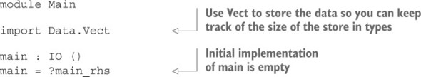
4.3.1. Representing the store
The data store itself is, initially, a collection of strings. We’ll begin by defining a type for the store, including the size of the store (that is, the number of stored items), explicitly and using a Vect for the items, as shown in the following listing. You can add this to DataStore.idr, above the initial empty definition of main.
Listing 4.14. A data type for representing the data store (DataStore.idr)
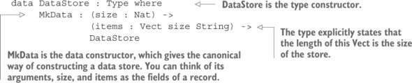
You can access the size and content of a data store by writing functions that pattern match on the data store and extract the appropriate fields. These are shown in the following listing.
Listing 4.15. Projecting out the size and content of a data store (DataStore.idr)
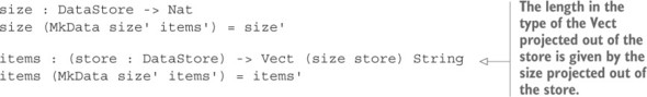
In this listing, the length of the Vect in the type of items is calculated by a function, size.
Records
A data type with one constructor, like DataStore, is essentially a record with fields for its data. In chapter 6, you’ll see a more concise syntax for records that avoids the need to write explicit projection functions such as size and items.
You’ll also need to add new data items to the store, as in listing 4.16. This adds items to the end of the store, rather than at the beginning using :: directly. The reason for this is that we plan to access items by their integer index; if you add items at the beginning, new items will always have an index of zero, and everything else will be shifted along one place.
Listing 4.16. Adding a new entry to the data store (DataStore.idr)
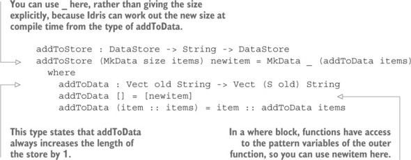
addToStore : DataStore -> String -> DataStore addToStore (MkData size items) newitem = MkData _ (addToData items) where addToData : Vect old String -> Vect (S old) String
You can use Ctrl-Alt-A to add a definition for addToData, and expression search with Ctrl-Alt-S is aware that newitem is in scope.
4.3.2. Interactively maintaining state in main
When you implement the main function for your data store, you’ll need to read input from the user, maintain the state of the store itself, and allow the user to exit. In the last chapter, we used the Prelude function repl to write a simple interactive program that repeatedly read input, ran a function on it, and displayed the output:
repl : String -> (String -> String) -> IO ()
Unfortunately, this only allows simple interactions that repeat forever.
For more-complex programs that maintain state, the Prelude provides another function, replWith, which implements a read-eval-print loop that carries some state. :doc describes it as follows:
Idris> :doc replWith Prelude.Interactive.replWith : (state : a) -> (prompt : String) -> (onInput : a -> String -> Maybe (String, a)) -> IO () A basic read-eval-print loop, maintaining a state Arguments: state : a -- the input state prompt : String -- the prompt to show onInput : a -> String -> Maybe (String, a) -- the function to run on reading input, returning a String to output and a new state. Returns Nothing if the repl should exit
On each iteration through the loop, it calls the onInput argument, which itself takes two arguments:
- The current state, of some generic type a
- The String entered at the prompt
The value the onInput function should return is of type Maybe (String, a), meaning that it can be in one of the following forms:
- Nothing, if it wants the loop to exit
- Just (output, newState), if it wants to print some output and update the state to newState for the next iteration
The next listing shows a simple example of this in action: an interactive program that reads an integer from the console and displays a running total of the sum of the inputs. If it reads a negative value, it will exit.
Listing 4.17. Interactive program to sum input values until a negative value is read (SumInputs.idr)
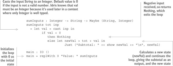
You can use replWith to refine the main function in the data store. At this stage you have
- A type for the data store (DataStore)
- A way of accessing the items in the store (items)
- A way of updating the store with new items (addToStore)
main : IO () main = replWith (MkData _ []) "Command: " ?processInput
Lifting processInput shows the type you have to work with:
processInput : DataStore -> String -> Maybe (String, DataStore) main : IO () main = replWith (MkData _ []) "Command: " processInput
Following the type-driven approach, when you refined the definition of main with an application of replWith, Idris was able to work out the necessary specialized type for processInput.
4.3.3. Commands: parsing user input
To process the String input, you somehow have to work out which one of the commands add, get, or quit has been entered. Rather than processing the input string directly, it’s usually much cleaner to define a new data type that represents the possible commands. This way, you can cleanly separate the parsing of commands from the processing.
You’ll therefore define a Command data type, which is a union type representing the possible commands and their arguments. Put the following definition in DataStore.idr above processInput:
data Command = Add String | Get Integer | Quit
Avoid using strings for data representation
The user enters a String, but only a certain number of Strings are valid input commands. Introducing the Command type makes the representation of commands more precise in that only valid commands can be represented. If the user enters a String that can’t be converted to a Command, the types force you to think about how to handle the error. At first, you can leave a hole in the program for error handling, but, ultimately, making a precise type leads to a more robust implementation.
You need to convert the string input by the user into a Command. The input may be invalid, however, so the type of the function to parse the command captures this possibility in its type:
parse : (input : String) -> Maybe Command
You can write a simple parser for input commands by searching for the first space in the input using the span function to establish which part of the input is the command and which is the argument. The span function works as follows:
Idris> :t Strings.span span : (Char -> Bool) -> String -> (String, String) Idris> span (/= ' ') "Hello world, here is a string" ("Hello", " world, here is a string") : (String, String) The first argument, (/= ' '), is a test that returns a Bool. This test returns True for any character that’s not equal to a space. The second argument is an input string, and span will split the string into two parts:
- The first part is the prefix of the input string, where all characters satisfy the test.
- The second part is the remainder of the string. If all characters in the string satisfy the test, this will be empty.
You can define parse with Ctrl-Alt-A and then refine its definition to the following:
parse : (input : String) -> Maybe Command parse input = case span (/= ' ') input of (cmd, args) => ?parseCommand
You can then lift parseCommand to a top-level function with the appropriate type, using Ctrl-Alt-L:
parseCommand : (cmd : String) -> (args : String) -> (input : String) -> Maybe Command parse : (input : String) -> Maybe Command parse input = case span (/= ' ') input of (cmd, args) => parseCommand cmd args input
You won’t need the input argument because you’ll be parsing the input from cmd and args alone, although Idris has added it because input is in scope. You can therefore edit the type:
parseCommand : (cmd : String) -> (args : String) -> Maybe Command parse : (input : String) -> Maybe Command parse input = case span (/= ' ') input of (cmd, args) => parseCommand cmd args
Also, you can see that args, if it’s not empty, will have a leading space, because the first character that span encounters that doesn’t satisfy the test will be a space. You can remove leading spaces with the ltrim : String -> String function, which returns its input with leading whitespace characters removed:
parseCommand : (cmd : String) -> (args : String) -> Maybe Command parse : (input : String) -> Maybe Command parse input = case span (/= ' ') input of (cmd, args) => parseCommand cmd (ltrim args)
You can now write parseCommand by examining the cmd and args arguments. You’ll need some Prelude functions to complete the definition of parseCommand:
- unpack : String -> List Char converts a String into a list of characters.
- isDigit : Char -> Bool returns whether a Char is one of the digits 0–9.
- all : (a -> Bool) -> List a -> Bool returns whether every entry in a list satisfies a test.
Thus, the expression all isDigit (unpack val) returns whether the string val consists entirely of digits.
Documentation and Prelude functions
In general, remember that you can use :doc at the REPL, or Ctrl-Alt-D in Atom, to check the documentation for any names, no matter whether they are type constructors, data constructors, or functions.
Listing 4.18 shows how parsing the input works. In particular, notice that pattern matching is very general; as long as patterns are composed of primitive ways of constructing a type (data constructors and primitive values), they are valid. An underscore is a match-anything pattern.
Listing 4.18. Parsing a command and argument string into a Command (DataStore.idr)
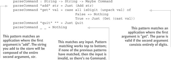
Now that you can parse a string into a Command, you can make more progress with processInput, calling parse. If it fails, you display an error message and leave the store as it is. Otherwise, you add a hole for processing the Command:
processInput : DataStore -> String -> Maybe (String, DataStore) processInput store inp = case parse inp of Nothing => Just ("Invalid command\n", store) Just cmd => ?processCommand 4.3.4. Processing commands
One way to proceed with your implementation of processInput would be to case-split on cmd and process the commands directly:processInput : DataStore -> String -> Maybe (String, DataStore) processInput store inp = case parse inp of Nothing => Just ("Invalid command\n", store) Just (Add item) => ?processCommand_1 Just (Get pos) => ?processCommand_2 Just Quit => ?processCommand_3 You can refine the implementation by filling in the easier holes, in the cases for Add item and Quit. The next listing shows how these holes are refined, leaving processCommand_2 for the moment.
Listing 4.19. Processing the inputs Add item and Quit (DataStore.idr)
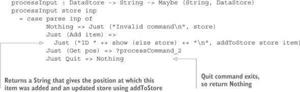
It’s always a good idea to inspect the types of holes Idris has generated to see what variables you have available, what their types are, and what type you need to build. For ?processCommand_2, you have this:
pos : Integer store : DataStore input : String -------------------------------------- processCommand_2 : Maybe (String, DataStore)
This will be slightly more involved than the other cases. You need to do the following:
- Get the items from the store.
- Ensure that the position, pos, is in range.
- If it is, extract the item from the specified pos and return it along with the store itself.
The type-define-refine process encourages you to write parts of definitions, step by step, constantly type-checking as you go, and constantly inspecting the types of the holes.
Because there are a few details involved in filling the ?processCommand_2 hole, we’ll rename it ?getEntry and lift it to a top-level function before implementing it step by step:
- Type— Lift getEntry to a new top-level function:
getEntry : (pos : Integer) -> (store : DataStore) -> (input : String) -> Maybe (String, DataStore)
- Define— Create a new skeleton definition:
getEntry pos store input = ?getEntry_rhs
- Define— You’ll need the items in the store, so define a new local variable for these:
getEntry pos store input = let store_items = items store in ?getEntry_rhs
Inspecting the type of getEntry_rhs tells you the type of store_items:pos : Integer store : DataStore input : String store_items : Vect (size store) String -------------------------------------- getEntry_rhs : Maybe (String, DataStore)
- Refine— To retrieve an entry from a Vect, you can use index as you’ve previously seen:
index : Fin n -> Vect n a -> a
To extract an entry from store_items, which has type Vect (size store), you’ll need a Fin (size store). Unfortunately, all you have available at the moment is an Integer. Using integerToFin, as described in section 4.2.3, you can refine the definition. If integerToFin returns Nothing, the input was out of bounds.getEntry : (pos : Integer) -> (store : DataStore) -> (input : String) -> Maybe (String, DataStore) getEntry pos store input = let store_items = items store in case integerToFin pos (size store) of Nothing => Just ("Out of range\n", store) Just id => ?getEntry_rhs_2 - Refine— If you inspect the type of getEntry_rhs_2 now, you’ll see that you have the Fin (size store) you need:
store : DataStore id : Fin (size store) pos : Integer input : String store_items : Vect (size store) String -------------------------------------- getEntry_rhs_2 : Maybe (String, DataStore)
You can now refine to a complete definition:getEntry : (pos : Integer) -> (store : DataStore) -> (input : String) Maybe (String, DataStore) getEntry pos store input = let store_items = items store in case integerToFin pos (size store) of Nothing => Just ("Out of range\n", store) Just id => Just (index id store_items ++ "\n", store) - Refine— As a final refinement, observe that input is never used, so you can remove this argument. Don’t forget to remove it from the application of get-Entry in processInput too.
getEntry : (pos : Integer) -> (store : DataStore) -> Maybe (String, DataStore) getEntry pos store = let store_items = items store in case integerToFin pos (size store) of Nothing => Just ("Out of range\n", store) Just id => Just (index id store_items ++ "\n", store)
By using a Vect for the store, with its size as part of the type, the type system can ensure that any access of the store by index will be within bounds, because you have to show that the index has the same upper bound as the length of the Vect.
For reference, the complete implementation of the data store is given in the following listing, with all the functions we just worked through.
Listing 4.20. Complete implementation of a simple data store (DataStore.idr)
module Main import Data.Vect data DataStore : Type where MkData : (size : Nat) -> (items : Vect size String) -> DataStore size : DataStore -> Nat size (MkData size' items') = size' items : (store : DataStore) -> Vect (size store) String items (MkData size' items') = items' addToStore : DataStore -> String -> DataStore addToStore (MkData size store) newitem = MkData _ (addToData store) where addToData : Vect oldsize String -> Vect (S oldsize) String addToData [] = [newitem] addToData (x :: xs) = x :: addToData xs data Command = Add String | Get Integer | Quit parseCommand : String -> String -> Maybe Command parseCommand "add" str = Just (Add str) parseCommand "get" val = case all isDigit (unpack val) of False => Nothing True => Just (Get (cast val)) parseCommand "quit" "" = Just Quit parseCommand _ _ = Nothing parse : (input : String) -> Maybe Command parse input = case span (/= ' ') input of (cmd, args) => parseCommand cmd (ltrim args) getEntry : (pos : Integer) -> (store : DataStore) -> Maybe (String, DataStore) getEntry pos store = let store_items = items store in case integerToFin pos (size store) of Nothing => Just ("Out of range\n", store) Just id => Just (index id (items store) ++ "\n", store) processInput : DataStore -> String -> Maybe (String, DataStore) processInput store input = case parse input of Nothing => Just ("Invalid command\n", store) Just (Add item) => Just ("ID " ++ show (size store) ++ "\n", addToStore store item) Just (Get pos) => getEntry pos store Just Quit => Nothing main : IO () main = replWith (MkData _ []) "Command: " processInput Exercises
- Add a size command that displays the number of entries in the store.
- Add a search command that displays all the entries in the store containing a given substring. Hint: Use Strings.isInfixOf.
- Extend search to print the location of each result, as well as the string. You can test your solution at the REPL as follows:
*ex_4_3> :exec Command: add Shearer ID 0 Command: add Milburn ID 1 Command: add White ID 2 Command: size 3 Command: search Mil 1: Milburn
4.4. Summary
- Data types are defined in terms of a type constructor and data constructors.
- Enumeration types are defined by listing the data constructors of the type.
- Union types are defined by listing the data constructors of the type, each of which may carry additional information.
- Generic types are parameterized over some other type. In a generic type definition, variables stand in place of concrete types.
- Dependent types can be indexed over any other value.
- Using dependent types, you can classify a larger family of types (such as vehicles) into smaller subgroups (such as vehicles powered by petrol and those powered by pedal) in the same declaration.
- Dependent types allow safety checks to be guaranteed at compile time, such as guaranteeing that all vector accesses are within the bounds of the vector.
- You can write larger programs in the type-driven style, creating new data types where appropriate to help describe components of the system.
- Interactive programs that involve state can be written using the replWith function.
Chapter 5. Interactive programs: input and output processing
This chapter covers
- Writing interactive console programs
- Distinguishing evaluation and execution
- Validating user inputs to dependently typed functions
Idris is a pure language, meaning that functions don’t have side effects, such as updating global variables, throwing exceptions, or performing console input or output. Realistically, though, when we put functions together to make complete programs, we’ll need to interact with users somehow.
In the preceding chapters, we used the repl and replWith functions to write simple, looping interactive programs that we can compile and execute without worrying too much about how they work. For all but the simplest programs, however, this approach is very limiting. In this chapter, you’ll see how interactive programs work in Idris more generally. You’ll see how to process and validate user input, and how you can write interactive programs that work with dependent types.
The key idea that allows us to write interactive programs in Idris, despite it being a pure language, is that we distinguish between evaluation and execution. We write interactive programs using a generic type IO, which describes sequences of actions that are then executed by the Idris runtime system.5.1. Interactive programming with IO
Although you can’t write functions that interact with a user directly, you can write functions that describe sequences of interactions. Once you have a description of a sequence of interactions, you can pass it to the Idris runtime environment, which will execute those actions.
The Prelude provides a generic type, IO, that allows you to describe interactive programs that return a value:
Idris> :doc IO IO : (res : Type) -> Type Interactive programs, describing I/O actions and returning a value. Arguments: res : Type -- The result type of the program
Thus, you distinguish in the type between functions that describe interactions with a user, and functions that return a value directly.
For example, consider the difference between the function types String -> Int and String -> IO Int:
- String -> Int is the type of a function that takes a String as an input and returns an Int without any user interaction or side effects.
- String -> IO Int is the type of a function that takes a String as an input and returns a description of an interactive program that produces an Int.
These are a couple of examples of functions with these types:
- length : String -> Int, which is defined in the Prelude, returns the length of the input String.
- readAndGetLength : String -> IO Int returns a description of interactive actions that display the input String as a prompt, reads another String from the console, and then returns the length of that String.
As you’ve seen in earlier chapters, the entry point to an Idris application is main : IO (), and we’ve used this to write simple interactive loops using the repl and replWith functions without worrying too much about the details of how these functions work. It’s now time to look at IO in more detail, and to learn how to write more-complex interactive programs.
Listing 5.1 shows an example of an interactive program that returns a description of the actions to display a prompt, read a user’s name, and then display a greeting. We’ll cover the details of the syntax throughout this section, but for now, notice the type of main : IO (). This type states that main takes no input and returns a description of interactive actions that produce an empty tuple.
Listing 5.1. A simple interactive program, reading a user’s name and displaying a greeting (Hello.idr)
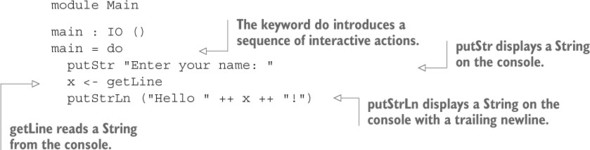
IO in Haskell and Idris
If you’re already familiar with Haskell, you’ll find that programming with IO in Idris is very similar to writing interactive programs in Haskell. If you understand listing 5.1, you can safely move on to section 5.3, where you’ll see how to validate user input and deal with errors in interactive Idris programs. You may also want to look at section 5.2.2, which discusses pattern-matching bindings.In this section, you’ll learn how to write interactive programs like this using IO in Idris and explore the distinction between evaluating expressions and executing programs, which allows us to write interactive programs without compromising on purity.
5.1.1. Evaluating and executing interactive programs
Functions that return an IO type are still considered pure, because they merely describe interactive actions. For example, the putStrLn function is defined in the Prelude and returns the actions that output a given String, plus a newline character, to the console:
Idris> :t putStrLn putStrLn : String -> IO ()
When you enter an expression at the REPL, Idris evaluates that expression. If that expression is a description of interactive actions, then to perform those actions requires an additional step, execution.
Figure 5.1 illustrates what happens when the expression putStrLn (show (47 * 2)) is executed. First, Idris calculates that the interactive action is to display "94\n" on the console (that is, the evaluator calculates the exact string that is to be displayed), and then it passes that action to the runtime environment.
Figure 5.1. Evaluating the expression putStrLn (show (47 * 2)) and then executing the resulting actions
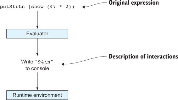
You can see what happens by evaluating the expression putStrLn (show (47 * 2)) at the REPL. This merely shows a description of the actions that a runtime environment can execute. There’s no need to look closely at the exact form of the result here, but you can at least see that the evaluation produces an expression with type IO ():
Idris> putStrLn (show (47 * 2)) io_bind (prim_write "94\n") (\__bindx => io_return ()) : IO ()
If you want to execute the resulting actions, you’ll need to pass this description to the Idris runtime environment. You achieve this with the :exec command at the REPL:
Idris> :exec putStrLn (show (47 * 2)) 94
In general, the :exec command, given an expression of type IO (), can be understood to do the following:
- Evaluate the expression, producing a description of the interactive actions to execute. In figure 5.1, evaluating the expression produces a description of an action: Write the string "94\n" to the console.
- Pass the resulting actions to the runtime environment, which executes them. In figure 5.1, executing the actions writes the string "94\n" to the console.
It’s also possible to compile to a standalone executable using the :c command at the REPL, which takes the executable name as an argument and generates a program that executes the actions described in main. For example, let’s go back to listing 5.1, repeated here:
module Main main : IO () main = do putStr "Enter your name: " x <- getLine putStrLn ("Hello " ++ x ++ "!") If you save this in a file, Hello.idr, and load it at the REPL, you can produce an executable as follows:
*Hello> :c hello
This results in an executable file called hello (or, on Windows systems, hello.exe) that can be run directly from the shell. For example:
$ ./hello Enter your name: Edwin Hello Edwin!Here, main describes not just one action but a sequence of actions. In general, in interactive programs you need to be able to sequence actions and have commands react to user input. Therefore, Idris provides facilities for combining smaller interactive programs into larger ones. We’ll begin by seeing how to do this using a Prelude function, (>>=), and then we’ll look at the higher-level syntax we used earlier in listing 5.1, the do notation.
5.1.2. Actions and sequencing: the >>= operator
In the brief example in listing 5.1, we used three IO actions:
- putStr : String -> IO (), which is an action to display a String on the console
- putStrLn : String -> IO (), which is an action to display a String followed by a newline on the console
- getLine : IO String, which is an action to read a String from the console
In order to write realistic programs, you’ll need to do more than just execute actions. You’ll need to be able to sequence actions, and you’ll need to be able to process the results of those actions.
Let’s say, for example, you want to read a string from the console and then output its length. There’s a length function in the Prelude, of type String -> Int, that you can use to calculate the length of a string, but getLine returns a value of type IO String, not String. The type IO String is a description of an action that produces a String, not the String itself.
In other words, you can get access to the string read from the console when the actions resulting from the function are executed, but you don’t yet have access to it when the function is evaluated. There’s no function of type IO String -> String. If such a function existed, it would mean that it was possible to know which string was read from the console without actually reading any string from the console!
The Prelude provides a function called >>= (intended to be used as an infix operator) that allows the sequencing of IO actions, feeding the result of one action as input into the next. It has the following type:
(>>=) : IO a -> (a -> IO b) -> IO b
Figure 5.2 shows an example application of >>= to sequence two actions, feeding the output of the first, getLine, as the input into the second, putStrLn. Because getLine returns a value of type IO String, Idris expects that putStrLn takes a String as its argument.
Figure 5.2. An interactive operation to read a String and then echo its contents using the >>= operator. The types of each subexpression are indicated.
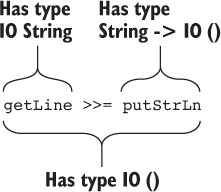
You can execute any sequence of actions with type IO () at the REPL using the :exec command, so you can execute the operations in figure 5.2 as follows:

To illustrate further, let’s try using >>= to write a printLength function that reads a string from the console and then outputs its length. To do this, take the following steps:
- Type— Our printLength function takes no input and returns a description of IO actions, so give it the following type:
printLength : IO ()
- Define— The function has a skeleton definition that takes no arguments:
printLength : IO () printLength = ?printLength_rhs
- Refine— Refine the printLength_rhs hole to call getLine for a description of an action that reads from the console, and use >>= to pass the value produced by getLine when it’s executed to the next action. Leave a hole in place of the next action for the moment:
printLength : IO () printLength = getLine >>= ?printLength_rhs
- Type— If you inspect the type of ?printLength_rhs, you’ll see that it has a function type:
-------------------------------------- printLength_rhs : String -> IO ()
The String in the function type here is the value that will be produced by executing getLine. This string will be available when the action is executed, and you can use it to compute the remaining IO actions. - Refine— An expression search on ?printLength_rhs will give you an anonymous function:
printLength : IO () printLength = getLine >>= \result => ?printLength_rhs1
The variable result is the String produced by the getLine action. Rename this to something more informative, like input:printLength : IO () printLength = getLine >>= \input => ?printLength_rhs1
- Refine— Because input is a String, you can use length to calculate its length as a Nat. Use a let binding to store this in a local variable:
printLength : IO () printLength = getLine >>= \input => let len = length input in ?printLength_rhs1
- Refine— Finally, complete the definition using show to convert len to a String, and putStrLn to give an action that displays the result:
printLength : IO () printLength = getLine >>= \input => let len = length input in putStrLn (show len)
You can try this definition at the REPL with :exec printLength, telling Idris that you’d like to execute the resulting actions rather than merely evaluate the expression:

Listing 5.2 shows the complete definition, further refined by displaying a prompt. The layout has also been adjusted in this definition to highlight the sequence of actions.
Listing 5.2. A function to display a prompt, read a string, and then display its length, using >>= to sequence IO actions (PrintLength.idr)
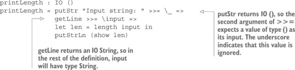
If you check the type of >>= at the REPL, you’ll see a constrained generic type:
Idris> :t (>>=) (>>=) : Monad m => m a -> (a -> m b) -> m b
In practice, this means that the pattern applies more generally than for IO, and you’ll see more of this later. For now, just read the type variable m here as IO.
In principle, you can always use >>= to sequence IO actions, feeding the output of one action as the input to the next. However, the resulting definitions are somewhat ugly, and sequencing actions is particularly common. That’s why Idris provides an alternative syntax for sequencing IO actions, the do notation.
5.1.3. Syntactic sugar for sequencing with do notation
Interactive programs are, by their nature, typically imperative in style, with a sequence of commands, each of which produces a value that can be used later. The >>= function captures this idea, but the resulting definitions can be difficult to read.
Instead, you can sequence IO actions inside do blocks, which allow you list the actions that will be run when a block is executed. For example, to print two things in succession you’d do something like this:
printTwoThings : IO () printTwoThings = do putStrLn "Hello" putStrLn "World"
Idris translates the do notation into applications of >>=. Figure 5.3 shows how this works in the simplest case, where an action is to be executed, followed by more actions.
Figure 5.3. Transforming do notation to an expression using the >>= operator when sequencing actions. The value produced by the action, of type ty, is ignored, as indicated by the underscore.
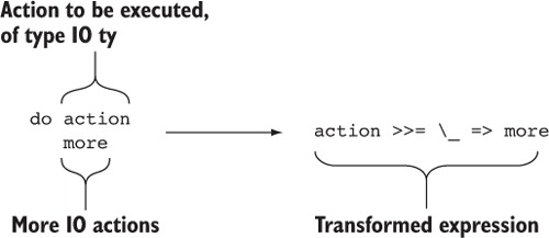
The result of an action can be assigned to a variable. For example, to assign the result of reading from the console with getLine to a variable x and then print the result, you can write this:
printInput : IO () printInput = do x <- getLine putStrLn x
The notation x <- getLine states that the result of the getLine action (that is, the String produced by the action of type IO String) will be stored in the variable x, which you can use in the rest of the do block. Sequencing actions and binding a variable like this with do notation directly translates to applications of >>=, as illustrated in figure 5.4.
Figure 5.4. Transforming do notation to an expression using the >>= operator, when binding a variable and sequencing actions
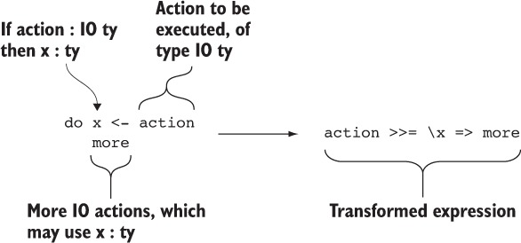
You can also use let inside do blocks to assign a pure expression to a variable. The following listing shows how printLength could be written using do notation instead of using >>= directly.
Listing 5.3. A function to display a prompt, read a string, and then display its length using do notation to sequence IO actions (PrintLength.idr)
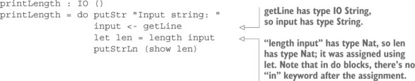
The printLength function in listing 5.3 uses two different forms for assigning to variables: using let and using <-. There’s an important difference between these two, which again relies on the distinction between evaluation and execution:
- Use let x = expression to assign the result of the evaluation of an expression to a variable.
- Use x <- action to assign the result of the execution of an action to a variable.
In listing 5.3, getLine describes an action, so it needs to be executed and the result assigned using <-, but length input doesn’t, so it’s assigned using let.
Most interactive definitions in Idris are written using do notation to control sequencing. In larger programs, you’ll also need to respond to user input and direct program flow. In the next section, we’ll look at various methods of reading and responding to user input, and at how to implement loops and other forms of control flow in interactive programs.
Exercises
- Using do notation, write a printLonger program that reads two strings and then displays the length of the longer string.
- Write the same program using >>= instead of do notation. You can test your answers at the REPL as follows:
*ex_5_1> :exec printLonger First string: short Second string: longer 6
5.2. Interactive programs and control flow
You’ve seen how to write basic interactive programs by sequencing existing actions, such as getLine to read input from the console and putStrLn to display text at the console. But as programs get larger, you’ll need more control: you’ll need to be able to validate and respond to user input, and you’ll need to express loops and other forms of control.In general, control flow in functions describing interactive actions works exactly the same way as control flow in pure functions, by pattern matching and recursion. Functions that describe interactive actions are pure functions themselves, after all, merely describing the actions that are to be executed later.
In this section, we’ll look at some common patterns that are encountered in interactive programs: producing pure values by combining the results of interactive actions, pattern matching on the results of interactive actions, and, finally, putting everything together in an interactive program with loops.
5.2.1. Producing pure values in interactive definitions
As well as describing actions for execution by the runtime system, you’ll often want to produce results from interactive programs. You’ve already seen getLine, for example:
getLine : IO String
The type IO String says that this is a function describing actions that produce a String as a result.
Often, you’ll want to write a function that uses an IO action such as getLine and then manipulates its result further before returning it. For example, you might want to write a readNumber function that reads a String from the console and converts it to a Nat if the input consists entirely of digits. It produces a value of type Maybe Nat:
- If the input consists entirely of digits representing the number i, it produces Just i. For example, on reading the string "1234", it produces Just 1234.
- Otherwise, it produces Nothing.
Listing 5.4 shows how to define readNumber. After reading an input using getLine, it checks whether every character in the input is a digit. If so, it converts the input to a Nat, producing a result using Just; otherwise, it produces Nothing.
Listing 5.4. Reading and validating a number (ReadNum.idr)
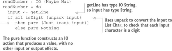
The pure function is used to produce a value in an interactive program without having any other input or output effects when it’s executed. Its purpose is to allow pure values to be constructed by interactive programs, as shown by its type:
pure : a -> IO a
To understand the need for pure in readNumber, you can replace the then and else branches of the if with holes, and inspect their types:
readNumber : IO (Maybe Nat) readNumber = do input <- getLine if all isDigit (unpack input) then ?numberOK else ?numberBad
If you look at the type of ?numberOK, you’ll see that you need a value of type IO (Maybe Nat):
input : String -------------------------------------- numberOK : IO (Maybe Nat)
You can then refine the ?numberOK and ?numberBad holes using pure:
readNumber : IO (Maybe Nat) readNumber = do input <- getLine if all isDigit (unpack input) then pure ?numberOK else pure ?numberBad
Now, if you look at the type of ?numberOK, you’ll see that you need a value of type Maybe Nat instead, without the IO wrapper:
input : String -------------------------------------- numberOK : Maybe Nat
As with >>=, if you check the type of pure at the REPL, you’ll see a constrained generic type, rather than a type that uses IO specifically:
Idris> :t pure pure : Applicative f => a -> f a
You can read the f here as IO. We’ll get to the exact meaning of Applicative and Monad in chapter 7; you don’t need to understand the details to write interactive programs.
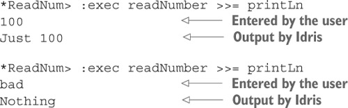
In the first case, the input is valid, so Idris produces the result Just 100. In the second case, the input has nondigit characters, so Idris produces Nothing.
printLn is a combination of putStrLn and show, and it’s convenient for displaying values at the console directly. It’s defined in the Prelude:
printLn : Show a => a -> IO () printLn x = putStrLn (show x)
5.2.2. Pattern-matching bindings
When an interactive action produces a value of some complex data type, such as readNumber, which produces a value of type Maybe Nat, you’ll often want to pattern-match on the intermediate result. You can do this using a case expression, but this can lead to deeply nested definitions. The following listing, for example, shows a function that reads two numbers from the console using readNumber, and produces a pair of those numbers if both are valid inputs, or Nothing otherwise.
Listing 5.5. Reading and validating a pair of numbers from the console (ReadNum.idr)
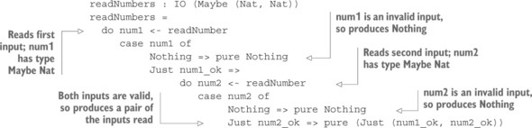
This will only get worse as functions get longer and there are more error conditions to deal with. To help with this, Idris provides some concise syntax for matching on intermediate values in do notation. First, we’ll take a look at a simple example, reading a pair of Strings from the console, and then we’ll revisit readNumbers and see how it can be made more concise.
You can write a function that reads two Strings and produces a pair as follows, using pure to combine the two inputs:
readPair : IO (String, String) readPair = do str1 <- getLine str2 <- getLine pure (str1, str2)
When you use the result produced by readPair, you’ll need to pattern-match on it to extract the first and second inputs. For example, to read a pair of Strings using readPair and then display both, you’d do this:
usePair : IO () usePair = do pair <- readPair case pair of (str1, str2) => putStrLn ("You entered " ++ str1 ++ " and " ++ str2) To make these programs more concise, Idris allows the pattern match and the assignment to be combined on one line, in a pattern-matching binding. The following program has exactly the same behavior as the preceding one:
usePair : IO () usePair = do (str1, str2) <- readPair putStrLn ("You entered " ++ str1 ++ " and " ++ str2) A similar idea works for readNumbers. You can pattern-match directly on the result of readNumber to check the validity of its result:
readNumbers : IO (Maybe (Nat, Nat)) readNumbers = do Just num1_ok <- readNumber Just num2_ok <- readNumber pure (Just (num1_ok, num2_ok))
This works as you’d like when the user enters valid numbers:
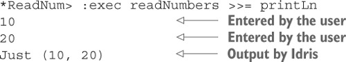
But, unfortunately, it doesn’t deal with the case where readNumber produces Nothing, and therefore crashes on execution:
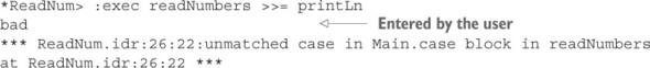
Idris has noticed this when checking readNumbers for totality:
*ReadNum> :total readNumbers_v2 Main.readNumbers is possibly not total due to: Main.case block in readNumbers at ReadNum.idr:26:22, which is not total as there are missing cases
Remember to check totality!
This incomplete definition of readNumbers illustrates why it’s important to check that functions are total. Even though readNumbers type-checks successfully, it could still fail at runtime due to the missing cases.Listing 5.6 shows how you can deal with the other possibilities in a pattern-matching binding. As well as the binding itself, you provide alternative matches after a vertical bar, showing how the rest of the function should proceed if the default match on Just num1_ok or Just num2_ok fails. This function has exactly the same behavior as the earlier function in listing 5.5.
Listing 5.6. Reading and validating a pair of numbers from the console, concisely (ReadNum.idr)
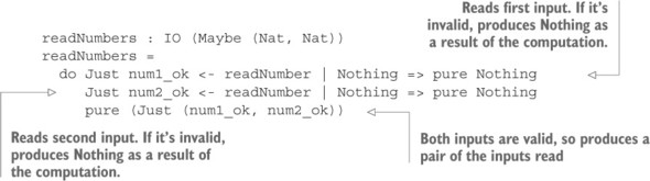
Pattern-matching bindings of this form allow you to express the expected valid behavior of a function in the default matches (Just num1_ok and Just num2_ok in listing 5.6), dealing with the error cases in the alternative matches.
5.2.3. Writing interactive definitions with loops
Now that you can read, validate, and respond to user input, let’s put everything together and write interactive definitions with loops.
You can write loops by writing recursive definitions. The next listing, for example, shows a countdown function that calculates a sequence of actions to display a countdown, with a one-second pause between displaying each number.
Listing 5.7. Display a countdown, pausing one second between each iteration (Loops.idr)
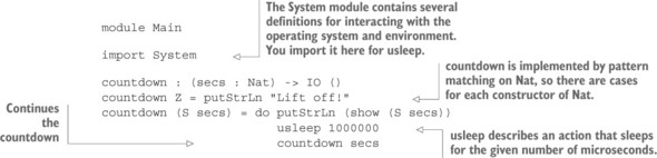
If you try executing this at the REPL using :exec, you’ll see a countdown displayed:
*Loops> :exec countdown 5 5 4 3 2 1 Lift off!
You can also check whether this function is total, that is, guaranteed to produce a result in finite time for all possible inputs:
*Loops> :total countdown Main.countdown is Total
In general, you can write an interactive function that describes a loop by making a recursive call to the function with its last action. In countdown, as long as the input argument isn’t Z, the program when executed will print the argument and wait a second before making a recursive call on the next smaller number. The number of iterations of the loop is therefore determined by the initial input. Because this is finite, countdown must terminate eventually, so Idris reports that it is total.
Totality and interactive programs
Totality checking is based on evaluation, not execution. The result of totality checking an IO program, therefore, tells you whether Idris will produce a finite sequence of actions, but nothing about the runtime behavior of those actions.
Sometimes, however, the number of iterations is determined by user input. For example, you can write a function to keep executing countdown until the user wants to stop, as shown next.
Listing 5.8. Keep running countdown until the user doesn’t want to run it any more (Loops.idr)
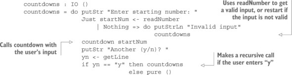
This function is not total, because there’s no guarantee that a user will ever enter anything other than y, or even provide any valid input.
*Loops> :total countdowns Main.countdowns is possibly not total due to recursive path: Main.countdownsInteractive programs that might loop forever, such as countdowns (or, more realistically, servers or operating systems) are not total, at least if we limit the definition to terminating programs. More precisely, a total function must either terminate or be guaranteed to produce a finite prefix of some infinite input, within finite time. We’ll discuss this further in chapter 11.
Exercises
- Write a function that implements a simple “guess the number” game. It should have the following type:
guess : (target : Nat) -> IO ()
Here, target is the number to be guessed, and guess should behave as follows:- Repeatedly ask the user to guess a number, and display whether the guess is too high, too low, or correct.
- When the guess is correct, exit.
- Implement a main function that chooses a random number between 1 and 100 and then calls guess. Hint: As a source of random numbers, you could use time : IO Integer, defined in the System module.
- Extend guess so that it counts the number of guesses the user has taken and displays that number before the input is read. Hint: Refine the type of guess to the following:
guess : (target : Nat) -> (guesses : Nat) -> IO ()
- Implement your own versions of repl and replWith. Remember that you’ll need to use different names to avoid clashing with the names defined in the Prelude.
5.3. Reading and validating dependent types
In previous chapters, you’ve seen several functions with dependent types, particularly using Vect to express lengths of vectors in their types. This allows you to state assumptions about the form of inputs to a function in its type and guarantees about the form of its output. For example, you’ve seen zip, which pairs corresponding elements of vectors:
zip : Vect n a -> Vect n b -> Vect n (a, b)
The type expresses the following:
- Assumption— Both input vectors have the same length, n.
- Guarantee— The output vector will have the same length as the input vectors.
- Guarantee— The output vector will consist of pairs of the element type of the first input vector and the element type of the second input vector.
Idris checks that whenever the function is called, the arguments satisfy the assumption and the definition of the function satisfies the guarantee.
So far, we’ve been testing functions such as zip at the REPL. Realistically, though, inputs to functions don’t come from such a carefully controlled environment where the Idris type checker is available. In practice, when a complete program is compiled and executed, inputs to functions will originate from some external source: perhaps a field on a web page, or user input at the console.
When a program reads data from some external source, it can’t make any assumptions about the form of that data. Rather, the program has to check that the data is of the necessary form. The type of a function tells you exactly what you need to check in order to evaluate it safely.
In this section, we’ll write a program that reads two vectors from the console, uses zip to pair corresponding elements if the vectors are the same length, and then displays the result. Although this is a simple goal, it demonstrates several important aspects of working with dependent types in interactive programs, and you’ll see many more examples of this form later in this book. You’ll see, briefly, how the types of the pure parts of programs tell you what you need to check in the interactive parts, and how the type system guides you toward the parts where error checking is necessary.
5.3.1. Reading a Vect from the console
As a first step, you’ll need to be able to read a vector from the console. Because vectors express their length in the type, you’ll need some way of describing the length of the vector you intend to read. One way is to take the length as an input, such as in the following type:
readVectLen : (len : Nat) -> IO (Vect len String)
This type states that readVectLen takes an intended length as input, and returns the sequence of actions that reads a vector of Strings of that length. The following listing shows one way you could implement this function.
Listing 5.9. Reading a Vect of known length from the console (ReadVect.idr)
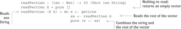
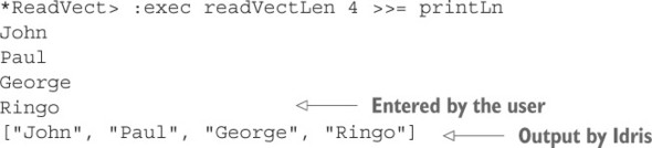
A problem with this approach is that you need to know in advance how long the vector should be, because the length is given as an input. What if, instead, you want to read strings until the user enters a blank line? You can’t know in advance how many strings the user will enter, so instead, you’ll need to return the length along with a vector of that length.
5.3.2. Reading a Vect of unknown length
If you read a vector from the console, terminated by a blank line, you can’t know how many elements will be in the resulting vector. In this situation, you can define a new data type that wraps not only the vector but also its length:
data VectUnknown : Type -> Type where MkVect : (len : Nat) -> Vect len a -> VectUnknown a
In type-driven development, we aim to express what we know about data in its type; if we can’t know something about data, we need to express this somehow too. This is the purpose of VectUnknown; it contains both the vector and its length, meaning that the length doesn’t have to be known in the type.
You can construct an example at the REPL:
*ReadVect> MkVect 4 ["John", "Paul", "George", "Ringo"] MkVect 4 ["John", "Paul", "George", "Ringo"] : VectUnknown String
In fact, you could leave an underscore in the expression instead of giving the length, 4, explicitly, because Idris can infer this from the length of the given vector:
*ReadVect> MkVect _ ["John", "Paul", "George", "Ringo"] MkVect 4 ["John", "Paul", "George", "Ringo"] : VectUnknown String
Having defined VectUnknown, instead of writing a function that returns IO (Vect len String), you can write a function that returns IO (VectUnknown String). That is, it returns not only the vector, but also its length:
readVect : IO (VectUnknown String)
This type states that readVect is a sequence of interactive actions that produce a vector of some unknown length, which will be determined at runtime. The following listing shows one possible implementation.
Listing 5.10. Reading a Vect of unknown length from the console (ReadVect.idr)
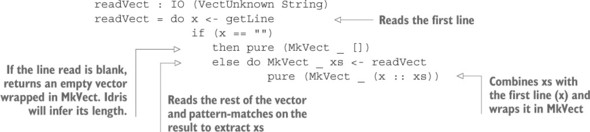
printVect : Show a => VectUnknown a -> IO () printVect (MkVect len xs) = putStrLn (show xs ++ " (length " ++ show len ++ ")")
Then, you can try reading some input at the REPL:
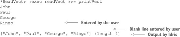
When dealing with user input, there’ll often be some properties of the data that you can’t know until runtime. The length of a vector is one example: once you’ve read the vector, you know its length, and from there you can check it and reason about how it relates to other data. But you could have a similar problem with any dependent data type that’s read from user input, and it would be better not to define a new type (like VectUnknown) every time this happens. Instead, Idris provides a more generic solution, dependent pairs.
5.3.3. Dependent pairs
You’ve already seen tuples, introduced in chapter 2, which allow you to combine values of different types, as in this example:
mypair : (Int, String) mypair = (94, "Pages")
A dependent pair is a more expressive form of this construct, where the type of the second element in a pair can be computed from the value of the first element. For example:
anyVect : (n : Nat ** Vect n String) anyVect = (3 ** ["Rod", "Jane", "Freddy"])
Dependent pairs are written with the elements separated by **. Their types are written using the same syntax as their values, except that the first element is given an explicit name (n in the preceding example). Figure 5.5 illustrates the syntax for dependent pair types.
Figure 5.5. Dependent pair syntax. Notice that the first element is given a name that can be used in the type of the second element.
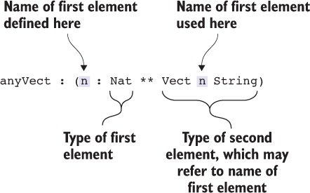
You can also often omit the type of the first element, if Idris can infer it from the type of the second element. For example:
anyVect : (n ** Vect n String) anyVect = (3 ** ["Rod", "Jane", "Freddy"])
If you replace the value ["Rod", "Jane", "Freddy"] with a hole, you can see how the first value, 3, affects its type:
anyVect : (n ** Vect n String) anyVect = (3 ** ?anyVect_rhs)
Inspecting the type of ?anyVect_rhs reveals that the second element must specifically be a vector of length 3, as specified by the first element:
-------------------------------------- anyVect_rhs : Vect 3 String
Types of subexpressions
Remember that when trying to understand larger program listings, you can replace subexpressions with a hole, like ?anyVect_rhs in the type-inference example, to find out their expected types and the types of any local variables that are in scope.
Instead of defining VectUnknown as in the section 5.3.2, you can define a function that reads vectors of unknown length by returning a dependent pair of the length, and a vector of that length. The following listing shows how readVect could be defined using dependent pairs.
Listing 5.11. Reading a Vect of unknown length from the console, returning a dependent pair (DepPairs.idr)
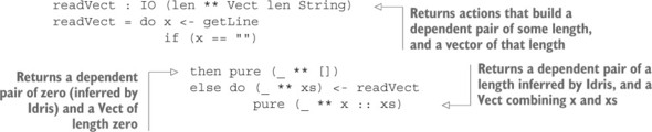
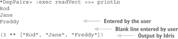
Now that you have the ability to read vectors of arbitrary and user-defined lengths from the console, we can complete our original goal of writing a program that reads two vectors and zips them together if their lengths match.
5.3.4. Validating Vect lengths
Our goal, as stated at the beginning of this section, is to write a program that does the following:
- Read two input vectors, using readVect.
- If they have different lengths, display an error.
- If they have the same lengths, display the result of zipping the vectors together.
The program will take its inputs from the user at the console and display its result on the console. We’ll implement it as a zipInputs function, as follows:
- Type— Because the input and output are entirely at the console, the type states that zipInputs takes no arguments and returns interactive actions:
zipInputs : IO ()
- Define— The first step in defining the function is to read two inputs using readVect. Leave a hole, ?zipInputs_rhs, for the rest of the definition:
zipInputs : IO () zipInputs = do putStrLn "Enter first vector (blank line to end):" (len1 ** vec1) <- readVect putStrLn "Enter second vector (blank line to end):" (len2 ** vec2) <- readVect ?zipInputs_rhs
- Type— Looking at the type of ?zipInputs_rhs, you can see the types (and hence the lengths) of the vectors that have been read:
len2 : Nat vec2 : Vect len2 String len1 : Nat vec1 : Vect len1 String -------------------------------------- zipInputs_rhs : IO ()
vec1 has length len1, and vec2 has length len2; there’s no explicit relationship between these lengths. Indeed, there shouldn’t be, because they were read independently. But if you look at the type of zip, you’ll see that the lengths must be the same before you can use it:zip : Vect n a -> Vect n b -> Vect n (a, b)
- Refine— Before you can make progress, you’ll need to check that the length of the second vector is the same as the length of the first. As a first attempt, you might try the following:
if len1 == len2 then ?zipInputs_rhs1 else ?zipInputs_rhs2
Unfortunately, this doesn’t help. If you look at the type of ?zipInputs_rhs1, you’ll see that nothing has changed:len1 : Nat len2 : Nat vec2 : Vect len2 String vec1 : Vect len1 String -------------------------------------- zipInputs_rhs1 : IO ()
The problem is that the type of len1 == len2, Bool, tells you nothing about the meaning of the operation itself. As far as Idris is concerned, the == operation could be implemented in any way (you’ll see in chapter 7 how == can be defined) and doesn’t necessarily guarantee that len1 and len2 really are equal. Instead, you can use the following function defined in Data.Vect:exactLength : (len : Nat) -> (input : Vect m a) -> Maybe (Vect len a)
This function takes a length, len, and a vector, input, of any length. If the length of the input vector turns out to be len, it returns Just input, with its type updated to Vect len a. Otherwise, it returns Nothing.Implementing exactLength
To implement exactLength, you need a more expressive type than Bool for representing the result of an equality test. You’ll see how to do this in chapter 8, and we’ll discuss the limitations of Bool in general.
Using exactLength, you can refine the definition as follows:zipInputs : IO () zipInputs = do putStrLn "Enter first vector (blank line to end):" (len1 ** vec1) <- readVect putStrLn "Enter second vector (blank line to end):" (len2 ** vec2) <- readVect case exactLength len1 vec2 of Nothing => ?zipInputs_rhs_1 Just vec2' => ?zipInputs_rhs_2
- Refine— For zipInputs_rhs_1, the inputs are different lengths, so you display an error:
case exactLength len1 vec2 of Nothing => putStrLn "Vectors are different lengths" Just vec2' => ?zipInputs_rhs_2
- Refine— For zipInputs_rhs_2, you have a new vector, vec2', which is the same as vec2 but with its length now guaranteed to be the same as the length of vec1, as you can confirm by looking at the type:
len1 : Nat vec2' : Vect len1 String len2 : Nat vec2 : Vect len2 String vec1 : Vect len1 String -------------------------------------- zipInputs_rhs_2 : IO ()
You can therefore complete the definition by calling zip with vec1 and vec2', and then printing the result:case exactLength len1 vec2 of Nothing => putStrLn "Vectors are different lengths" Just vec2' => printLn (zip vec1 vec2')
For reference, the complete definition is given in the following listing.
Listing 5.12. Complete definition of zipInputs (DepPairs.idr)
zipInputs : IO () zipInputs = do putStrLn "Enter first vector (blank line to end):" (len1 ** vec1) <- readVect putStrLn "Enter second vector (blank line to end):" (len2 ** vec2) <- readVect case exactLength len1 vec2 of Nothing => putStrLn "Vectors are different lengths" Just vec2' => printLn (zip vec1 vec2')
Exercises
In these exercises, you’ll find the following Prelude functions useful, in addition to the functions discussed earlier in the chapter: openFile, closeFile, fEOF, fGetLine, and writeFile. Use :doc to find out what each of these do. Also, see the sidebar, “Handling I/O errors.”
- Write a function, readToBlank : IO (List String), that reads input from the console until the user enters a blank line.
- Write a function, readAndSave : IO (), that reads input from the console until the user enters a blank line, and then reads a filename from the console and writes the input to that file.
- Write a function, readVectFile : (filename : String) -> IO (n ** Vect n String), that reads the contents of a file into a dependent pair containing a length and a Vect of that length. If there are any errors, it should return an empty vector.
Many of the functions in the Exercises may return errors using Either. At first, you can assume the result is successful using a pattern-matching binding, as described in section 5.2.2:
do Right h <- openFile filename Read Right line <- fGetLine h {- rest of code -} Then, to make the function total, handle errors using the notation described in the same section:
do Right h <- openFile filename Read | Left err => putStrLn (show err) Right line <- fGetLine h | Left err => putStrLn (show err) {- rest of code -} 5.4. Summary
- Idris provides a generic IO type for describing interactive actions.
- Idris distinguishes between evaluation of pure functions and execution of interactive actions. The :exec command at the REPL executes interactive actions.
- You can sequence interactive actions using do notation, which translates to applications of the >>= operator.
- You can produce pure values from interactive definitions by using the pure function.
- Idris provides a concise notation for pattern-matching on the result of an interactive action.
- Dependent types express assumptions about inputs to functions, so you need to validate user inputs to check that they satisfy those assumptions.
- Dependent pairs allow you to pair two values, where the type of the second value is computed from the first value.
- You can use dependent pairs to express that a type’s argument, such as the length of a vector, will not be known until the user enters some input.
Chapter 6. Programming with first-class types
This chapter covers- Programming with type-level functions
- Writing functions with varying numbers of arguments
- Using type-level functions to calculate the structure of data
- Refining larger interactive programs
In Idris, as you’ve seen several times now, types can be manipulated just like any other language construct. For example, they can be stored in variables, passed to functions, or constructed by functions. Furthermore, because they’re truly first-class, expressions can compute types, and types can also take any expression as an argument. You’ve seen several uses of this concept in practice, in particular the ability to store additional information about data in its type, such as the length of a vector.
In this chapter, we’ll explore more ways of taking advantage of the first-class nature of types. You’ll see how type-level functions can be used to give alternative names to types and also to calculate the type of a function from some other data. In
particular, you’ll see how you can write a type-safe formatted output function, printf. For printf, the type (and even number) of arguments to the function are calculated from a format string provided as its first argument. This technique, calculating the type of some data (in this case, the arguments to printf) based on some other data (in this case, the format string) is often useful. Here are a couple of examples:- Given an HTML form on a web page, you can calculate the type of a function to process inputs in the form.
- Given a database schema, you can calculate types for queries on that database.
As an example of this concept, you’ll see how to use type-level functions to refine the data store we implemented at the end of chapter 4. Previously, you could only store data as Strings, but for more flexibility you might want the form of the data to be described by a user rather than hardcoded into the program. Using type-level functions, you’ll extend the data store with a schema that describes the form of the data, and you’ll use that schema to calculate appropriate types for functions to parse and display user data. In doing so, you’ll learn more about using holes to help correct errors when refining larger programs.
To begin, we’ll look at how to use functions at the type level to calculate types.
6.1. Type-level functions: calculating types
One of the most fundamental features of Idris is that types and expressions are part of the same language—you use the same syntax for both. You’ve already seen in chapter 4 that expressions can appear in types. For example, in the type of append on Vect, we have n and m (both Nats), and the resulting length is n + m:
append : Vect n elem -> Vect m elem -> Vect (n + m) elem
Here, n, m, and n + m all have type Nat, which can also be used in ordinary expressions. Similarly, you can use types in expressions and therefore write functions that calculate types. There are two common situations where you might want to do this:
- To give more meaningful names to composite types— For example, if you have a type (Double, Double) representing a position as a 2D coordinate, you might prefer to call the type Position to make the code more readable and self-documenting.
- To allow a function’s type to vary according to some contextual information— For example, the type of a value returned by a database query will vary depending on the database schema and the query itself.
In the first case, you can define type synonyms, which give alternative names to types. In the second case, you can define type-level functions (of which type synonyms are a special case) that calculate types from some input. In this section, we’ll take a look at both.
6.1.1. Type synonyms: giving informative names to complex types
Let’s say you’re writing an application that deals with complex polygons, such as a drawing application. You might represent a polygon as a vector of the coordinates of each corner. A triangle, for example, might be initialized as follows:tri : Vect 3 (Double, Double) tri = [(0.0, 0.0), (3.0, 0.0), (0.0, 4.0)]
The type, Vect 3 (Double, Double) says exactly what the form of the data will be, which is useful to the machine, but it doesn’t give any indication to the reader what the purpose of the data is. Instead, you can refine the type using a type synonym for a position represented as a 2D coordinate:
Position : Type Position = (Double, Double)
Here, you have a function called Position that takes no arguments and returns a Type. This is an ordinary function; there’s nothing special about the way it’s declared or implemented. Now, anywhere you can use a Type, you can use Position to calculate that type. For example, the triangle can be defined with a refined type as follows:
tri : Vect 3 Position tri = [(0.0, 0.0), (3.0, 0.0), (0.0, 4.0)]
This kind of function is a type synonym because it provides an alternative name for some other type.
Naming convention
By convention, we usually use an initial capital letter for functions that are intended to compute types.
Because they’re ordinary functions, they can also take arguments. For example, the following listing shows how you can use type synonyms to express more clearly that the Vect is intended to represent a polygon.
Listing 6.1. Defining a polygon using type synonyms (TypeSynonym.idr)
Because Polygon is an ordinary function, you can evaluate it at the REPL:
*TypeSynonyms> Polygon 3 Vect 3 (Double, Double) : TypeAlso, notice that if you evaluate tri at the REPL, Idris will display tri’s type in the evaluated form. In other words, evaluation at the REPL evaluates both the expression and the type:
*TypeSynonyms> tri [(0.0, 0.0), (3.0, 0.0), (0.0, 4.0)] : Vect 3 (Double, Double)
Using :t, on the other hand, displays tri’s type:
*TypeSynonyms> :t tri Polygon 3
Finally, you can see what happens when you try to define tri interactively using expression search in Atom. Enter the following into an Atom buffer, along with the previous definition of Polygon:
tri : Polygon 3 tri = ?tri_rhs
The interactive editing tools in general, and expression search in particular, are aware of how type synonyms are defined, so if you try an expression search on tri_rhs, you’ll get the same result as if the type were written directly as Vect 3 (Double, Double):
tri : Polygon 3 tri = [(?tri_rhs1, ?tri_rhs2), (?tri_rhs3, ?tri_rhs4), (?tri_rhs5, ?tri_rhs6)]
The type synonyms defined in this section, Position and Polygon, are really just ordinary functions that happen to be used to compute types. This gives you a lot of flexibility in how you describe types, as you’ll see in the rest of this chapter.
6.1.2. Type-level functions with pattern matching
Type synonyms are a special case of type-level functions, which are functions that can be used anywhere Idris is expecting a Type. There isn’t anything special about type-level functions as far as Idris is concerned; they’re ordinary functions that happen to return a Type, and they can use all of the language constructs available elsewhere. Nevertheless, it’s useful to consider them separately, to see how they work in practice.
Because type-level functions are ordinary functions that return a type, you can write them by case splitting. For example, the following listing shows a function that calculates a type from a Boolean input. You saw this function in chapter 1, although in a slightly different form.
Listing 6.2. A function that calculates a type from a Bool (TypeFuns.idr)
StringOrInt : Bool -> Type StringOrInt False = String StringOrInt True = IntUsing this, you can write a function where the return type is calculated from or depends on an input. Using StringOrInt, you can write functions that return either type, depending on a Boolean flag.
As a small example, you can write a function that takes a Boolean input and returns the string "Ninety four" if it’s False, or the integer 94 if it’s True. Begin with the type:
- Type— Begin by giving a type declaration, using StringOrInt:
getStringOrInt : (isInt : Bool) -> StringOrInt isInt getStringOrInt isInt = ?getStringOrInt_rhs
If you look at the type of getStringOrInt_rhs now, you’ll see this:isInt : Bool -------------------------------------- getStringOrInt_rhs : StringOrInt isInt
- Define— Because isInt appears in the required type for getStringOrInt_rhs, case splitting on isInt will cause the expected return type to change according to the specific value of isInt for each case. Case splitting on isInt leads to this:
getStringOrInt : (isInt : Bool) -> StringOrInt isInt getStringOrInt False = ?getStringOrInt_rhs_1 getStringOrInt True = ?getStringOrInt_rhs_2
- Type— Looking at the types of the newly created holes, you can see how the expected type is changed in each case:
-------------------------------------- getStringOrInt_rhs_1 : String -------------------------------------- getStringOrInt_rhs_2 : Int
In getStringOrInt_rhs_1, the type is refined to StringOrInt False because the pattern for isInt is False, which evaluates to String. Then, in getString-OrInt_rhs_2, the type is refined to StringOrInt True, which evaluates to Int. - Refine— To complete the definition, you need to provide values of different types in each case:
getStringOrInt : (isInt : Bool) -> StringOrInt isInt getStringOrInt False = "Ninety four" getStringOrInt True = 94
Dependent pattern matching
The getStringOrInt example illustrates a technique that’s often useful when programming with dependent types: dependent pattern matching. This refers to a situation where the type of one argument to a function can be determined by inspecting the value of (that is, by case splitting) another. You’ve already seen an example of this when defining zip in chapter 4, where the form of one vector restricted the valid forms of the other, and you’ll see a lot more.
- If the input is a String, it returns the String with leading and trailing space removed using trim.
- If the input is an Int, it converts the input to a String using cast.
Documentation
Remember that you can use :t and :doc to check the types of functions that are unfamiliar (such as trim) at the REPL.
You can define this function with the following steps:
- Type— Begin by writing a type for valToString, again using StringOrInt, but this time to calculate the input type:
valToString : (isInt : Bool) -> StringOrInt isInt -> String valToString isInt y = ?valToString_rhs
Inspecting the type of valToString_rhs, you’ll see the following:isInt : Bool y : StringOrInt isInt -------------------------------------- valToString_rhs : String
- Define— You can define this by case splitting on isInt. The type of y is calculated from isInt, so if you case-split on isInt, you should see refined types for y in each resulting case:
valToString : (isInt : Bool) -> StringOrInt isInt -> String valToString False y = ?valToString_rhs_1 valToString True y = ?valToString_rhs_2
- Type— Inspecting the types of valToString_rhs_1 and valToString_rhs_2 shows how the type of y is refined in each case:
y : String -------------------------------------- valToString_rhs_1 : String y : Int -------------------------------------- valToString_rhs_2 : String
- Refine— To complete the definition, fill in the right side to convert y to a trimmed String if it was a String, or a string representation of the number if it was an Int:
valToString : (isInt : Bool) -> StringOrInt isInt -> String valToString False y = trim y valToString True y = cast y
There’s more that you can achieve with type-level expressions, however. The fact that types are first-class means not only that types can be computed like any other value, but also that any expression form can appear in types.
6.1.3. Using case expressions in types
Any expression that can be used in a function can also be used at the type level, and vice versa. For example, you can leave holes in types while your understanding of a function’s requirements develops, or you can use more-complex expression forms such as case. Let’s briefly take a look at how this can work by using a case expression in the type of valToString instead of a separate StringOrInt function:
- Type— Start by giving a type for valToString, but because you don’t immediately know the input type, you can leave a hole:
valToString : (isInt : Bool) -> ?argType -> String
- Define— Even though you have an incomplete type, you can still proceed with the definition by case splitting on isInt, because you at least know that isInt is a Bool:
valToString : (isInt : Bool) -> ?argType -> String valToString False y = ?valToString_rhs_1 valToString True y = ?valToString_rhs_2
- Type— Inspecting the types of valToString_rhs_1 and valToString_rhs_2 will, however, reveal that you don’t know the type of y yet:
y : ?argType -------------------------------------- valToString_rhs_1 : String
- Refine— At this stage, you need to refine the type with more details of ?argType. You can fill in ?argType with a case expression:
valToString : (isInt : Bool) -> (case _ of case_val => ?argType) -> String valToString False y = ?valToString_rhs_1 valToString True y = ?valToString_rhs_2
- Refine— Remember that when Idris generates a case expression, it leaves an underscore in place of the value the case expression will branch on. You’ll need to fill this in before the program will compile. You can compute the argument type from the input isInt:
valToString : (isInt : Bool) -> (case isInt of case_val => ?argType) -> String valToString False y = ?valToString_rhs_1 valToString True y = ?valToString_rhs_2
- Refine— Case splitting on case_val gives you the two possible values isInt can take:
valToString : (isInt : Bool) -> (case isInt of False => ?argType_1 True => ?argType_2) -> String valToString False y = ?valToString_rhs_1 valToString True y = ?valToString_rhs_2
You can then complete the type in the same way as your implementation of StringOrInt, refining ?argType_1 with String and ?argType_2 with Int:valToString : (isInt : Bool) -> (case isInt of False => String True => Int) -> String valToString False y = ?valToString_rhs_1 valToString True y = ?valToString_rhs_2
- Type— Inspecting ?valToString_rhs_1 and ?valToString_rhs2 now will show you the new types for the input y, calculated from the first argument:
y : String -------------------------------------- valToString_rhs_1 : String y : Int -------------------------------------- valToString_rhs_2 : String
- Refine— Finally, now that you know the type of the input y in each case, you can complete the definition as before:
valToString : (isInt : Bool) -> (case isInt of False => String True => Int) -> String valToString False y = trim y valToString True y = cast y
In general, it’s best to consider type-level functions in exactly the same way as ordinary functions, as we’ve done so far. This isn’t always the case, though. There are a couple of technical differences that are useful to know about:
- Type-level functions exist at compile time only. There’s no runtime representation of Type, and no way to inspect a Type directly, such as pattern matching.
- Only functions that are total will be evaluated at the type level. A function that isn’t total may not terminate, or may not cover all possible inputs. Therefore, to ensure that type-checking itself terminates, functions that are not total are treated as constants at the type level, and don’t evaluate further.
6.2. Defining functions with variable numbers of arguments
You can use type-level functions to calculate types based on some other known input. Given that function types are themselves types, this means that you can write functions with a different number of arguments depending on some other input. This is similar to some other languages that support variable-length argument lists, but with additional precision in the type because you use the value of one argument to compute the types of the others.In this section, we’ll see a couple of examples of how this can work:
- As an introductory example, we’ll write a function that adds a sequence of numbers, where the first argument is a number used to calculate the type of a function that takes that many inputs.
- We’ll use the same technique to write a variant of the printf function that produces a formatted output String using a format specifier in its first argument to describe the form of later arguments.
6.2.1. An addition function
First, we’ll define an addition function that adds together a sequence of numbers given directly as function arguments. Its behavior is characterized by the three examples shown in figure 6.1. An expression of the form adder numargs val calculates a function that takes numargs additional arguments, which are added to an initial value val.
Figure 6.1. Behavior of an addition function with a variable number of arguments
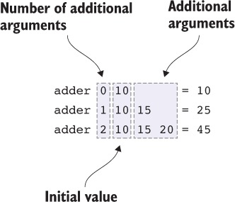
As usual in type-driven development, you’ll begin writing adder by writing its type, but in this case the type is not something you can construct directly; the type of adder is different depending on the value of the first argument. For the examples shown in figure 6.1, you’re looking for the following types:
adder 0 : Int -> Int adder 1 : Int -> Int -> Int adder 2 : Int -> Int -> Int -> Int ...
Because types are first-class, and this type differs depending on some value, you’ll be able to compute it using a type-level function. You can write an AdderType function with the required behavior. The name AdderType follows the convention that type-level functions are given names with an initial capital letter, and it indicates that it’s used to compute the type of adder.
You can use a Nat to give the length of the argument list, both because you can case-split on it conveniently, and because it would be meaningless to have a negative length argument list. The following listing gives the definition of AdderType.Listing 6.3. A function to calculate a type for adder n (Adder.idr)
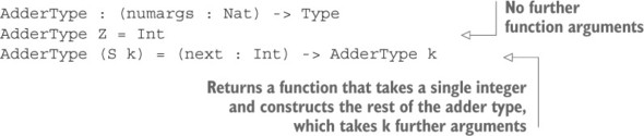
The type of adder can now be computed by passing its first argument to AdderType. The second argument is the initial value, which we’ll call acc as an abbreviation for “accumulator”:
adder : (numargs : Nat) -> (acc : Int) -> AdderType numargs
Because you calculate the type by case splitting on numargs in AdderType, you can write the definition of adder with a corresponding structure by case splitting on numargs, so that AdderType will be refined for each case. You can implement it with the following steps:
- Define— Add a skeleton definition, and then case-split on the first argument:
adder : (numargs : Nat) -> (acc : Int) -> AdderType numargs adder Z acc = ?adder_rhs_1 adder (S k) acc = ?adder_rhs_2
- Refine— Where the number of additional arguments, numargs, is Z, return the accumulator directly:
adder : (numargs : Nat) -> (acc : Int) -> AdderType numargs adder Z acc = acc adder (S k) acc = ?adder_rhs_2
- Type— For adder_rhs_2, inspecting the type of the hole shows that you need to provide a function:
k : Nat acc : Int -------------------------------------- adder_rhs_2 : Int -> AdderType k
This is a function type because in AdderType when numargs matches a nonzero Nat, the expected type is a function type. - Refine— The only way you have of producing something of type AdderType k in general is by calling adder with k as the first argument, so this type hints that you need to make a recursive call to adder. This is the complete definition:
adder : (numargs : Nat) -> (acc : Int) -> AdderType numargs adder Z acc = acc adder (S k) acc = \next => adder k (next + acc)
Listing 6.4 shows a slightly refined version of the adder function that works with any numeric type, not just Int. It does this by passing an additional Type argument to AdderType, and then constraining that to numeric types in the type of adder.
Listing 6.4. A generic adder that works for any numeric type (Adder.idr)
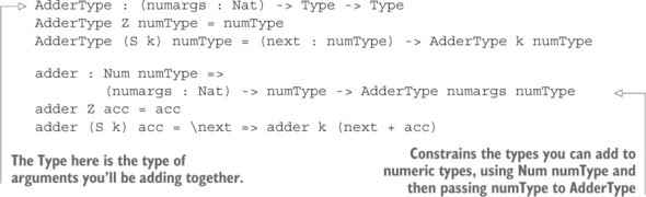
The adder function illustrates the basic pattern for defining functions with variable numbers of arguments: you’ve written an AdderType function to calculate the desired type of adder, given one of adder’s inputs. The pattern can also be applied for larger definitions, as you’ll now see when we define a function for formatting output.
6.2.2. Formatted output: a type-safe printf function
A larger example of a function with a variable number of arguments is printf, found in C and some other languages. It produces formatted output given a format string and a variable number of arguments, as determined by the format string. The format string essentially gives a template string to be output, populated by the remaining arguments. In essence, printf has the same overall structure as adder, using the format string to calculate the types of the later arguments.
Figure 6.2 shows some examples that characterize the printf behavior. Note that rather than producing output to the console, our version of printf returns a String.
Figure 6.2. Behavior of a printf function with different format strings
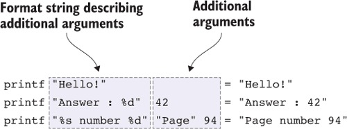
In these format strings, the directive %d stands for an Int; %s stands for a String; and anything else is printed literally.
Following our usual process of type, define, refine, we’ll begin by thinking about a type for printf. As with adder, we’ll start with the types of the characteristic examples and then work out how to write a function that computes these types. These are the types of the examples in figure 6.2:
printf "Hello!" : String printf "Answer: %d" : Int -> String printf "%s number %d" : String -> Int -> String
Format strings
In a full implementation of printf as provided by C, there are far more directives available than %d and %s. Furthermore, the directives can be modified in various ways to indicate further how the output should be formatted (such as leading zeroes in a number). Such details don’t add anything to this discussion of type-level functions, however, so we’ll omit them here.
To get the type of printf, you’ll need to use the format string to build the expected types of the arguments. Instead of processing the string directly, you can write a data type describing the possible formats, as follows.
Listing 6.5. Representing format strings as a data type (Printf.idr)
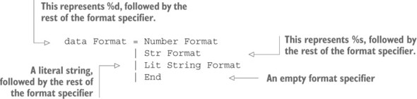
This gives a clean separation between the parsing of the format string and the processing, much as we did when parsing the commands to the data store in chapter 4. For example, Str (Lit " = " (Number End)) would represent the format string "%s = %d", as illustrated in figure 6.3.
Figure 6.3. Translating a format string to a Format description
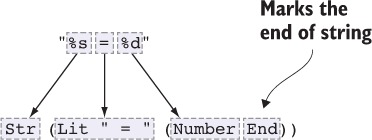
- The meaning of String is not obvious from the type alone. The function type Format -> Type has a more precise meaning than the function type String -> Type because it’s clear that the input must be a format specification rather than any String.
- Defining an intermediate data type gives us access to more interactive editing features, particularly case splitting.
For the moment, we’ll work directly with Format; we’ll define a conversion from String to Format later. The following listing shows how you can compute the type of printf from a Format specifier.
Listing 6.6. Calculating the type of printf from a Format specifier (extending Printf.idr)
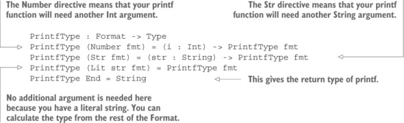
Listing 6.7 defines a helper function for building a String from a Format, along with any necessary additional arguments as calculated by PrintfType. This works like adder, using an accumulator to build the result.
Listing 6.7. Helper function for printf, building a String from a Format specifier (Printf.idr)
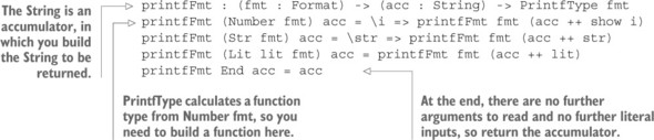
Remember interactive editing!
For examples such as those in listings 6.6 and 6.7, don’t just type them in directly. Instead, use the interactive editing tools in Atom to try to reconstruct them yourself. While doing so, make sure you take a look at the types of any holes, and see how far expression search can take you.Finally, to implement a printf that takes a String as a format specifier rather than a Format structure, you’ll need to be able to convert a String into a Format. The following listing defines the top-level printf function that does this conversion.
Listing 6.8. Top-level definition of printf, with a conversion from String to Format (Printf.idr)
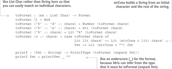
Exercises
- An n x m matrix can be represented by nested vectors of Double. Define a type synonym: Matrix : Nat -> Nat -> Type. You should be able to use it to define the following matrix:
testMatrix : Matrix 2 3 testMatrix = [[0, 0, 0], [0, 0, 0]]
- Extend printf to support formatting directives for Char and Double. You can test your answer at the REPL as follows:
*ex_6_2> :t printf "%c %f" printf "%c %f" : Char -> Double -> String *ex_6_2> printf "%c %f" 'X' 24 "'X' 24.0" : String
- You could implement a vector as nested pairs, with the nesting calculated from the length, as in this example:
TupleVect 0 ty = () TupleVect 1 ty = (ty, ()) TupleVect 2 ty = (ty, (ty, ())) ...
Define a type-level function, TupleVect, that implements this behavior. Remember to start with the type of TupleVect. When you have the correct answer, the following definition will be valid:test : TupleVect 4 Nat test = (1,2,3,4,())
6.3. Enhancing the interactive data store with schemas
In the interactive data store we developed in chapter 4, you were able to add Strings to an in-memory store and retrieve them by index. But what if you want to store more-complex data? And what if you’d like the form of the data to be determined by the user before entering any data, rather than by hardcoding it in the program itself?
In the rest of this chapter, we’ll extend the data store by adding schemas to describe the form of the data. We’ll determine the schema by user input, and we’ll use type-level functions to compute the correct type for the data. Figure 6.4 shows two different data stores, with different schemas, that we’ll be able to represent with our extended system. Schema 1, at the top, shows a store that requires the data to be of type (Int, String), and schema 2, below, shows a store that requires the data to be of type (String, String, Int). In contrast, in the data store developed in chapter 4, the schema was effectively always String.
Figure 6.4. Two different data stores, with different schemas. Schema 1 requires the data to be of type (Int, String), and schema 2 requires the data to be of type (String, String, Int)
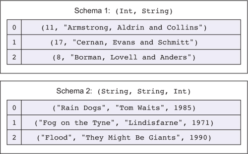
A typical interaction with the extended system might proceed as follows. Note that we’re describing the schema before entering any data.
Command: schema String String Int OK Command: add "Rain Dogs" "Tom Waits" 1985 ID 0 Command: add "Fog on the Tyne" "Lindisfarne" 1971 ID 1 Command: get 1 "Fog on the Tyne", "Lindisfarne", 1971 Command: quitRather than starting from scratch, we’ll begin with the existing data store we implemented in chapter 4 and refine the overall system as necessary. We’ll take this approach:
- Refine the representation of DataStore to include schema descriptions. This refinement will inevitably mean that our program no longer type-checks.
- Correct any errors, introducing holes for any more-complex errors.
- Fill in the holes to complete the implementation, and add any further features that are now supported as a result of refining the type.
6.3.1. Refining the DataStore type
At the moment, the DataStore only supports storing Strings. We implemented it in chapter 4 using the following type:
data DataStore : Type where MkData : (size : Nat) -> (items : Vect size String) -> DataStore
Instead of using a Vect size String for the items in the store, we’d like to be flexible in the types of these items. One natural way to do this might be to refine this to a generic version of DataStore, parameterizing it over a schema that gives the type of data in the store:
data DataStore : Type -> Type where MkData : (size : Nat) -> (items : Vect size schema) -> DataStore schema
Commenting out code sections
While you’re working on the refined DataStore, you’ll inevitably break the rest of the program, which will no longer type-check. Therefore, I’d suggest commenting out the rest of the code (placing it between {- and -}) until you’ve finished the new DataStore type and you’re ready to move on.
We want the user to be able to describe and possibly even update the schema, but if we parameterize over a schema type, the schema will be fixed in the type. Instead, we’ll create a data type for describing schemas, and a type-level function for translating schema descriptions (possibly given by a user at runtime) into concrete types. The following listing shows an outline of a refined DataStore type.
Listing 6.9. Outline of the refined DataStore type, with the Schema description and the translation of Schema to concrete types left undefined (DataStore.idr)
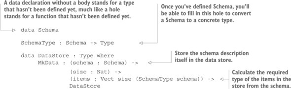
The next listing shows how you can describe Schemas and convert them into Idris Types using a type-level function, SchemaType.
Listing 6.10. Defining Schema, and converting a Schema to a concrete type
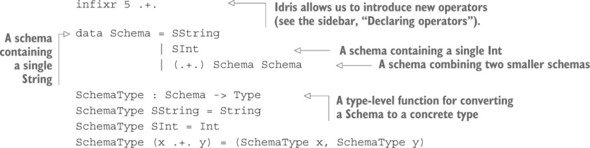
You can try this for defining schemas for the two example stores shown in figure 6.4 earlier:
*DataStore> SchemaType (SInt .+. SString) (Int, String) : Type *DataStore> SchemaType (SString .+. SString .+. SInt) (String, String, Int) : Type
You can define new operators by giving their fixity and precedence. In listing 6.10 you had this:
infixr 5 .+.
This introduces a new right-associative infix operator (infixr) with precedence level 5. In general, operators are introduced with the keyword infixl (for left-associative operators), infixr (for right-associative operators) or infix (for non-associative operators), followed by a precedence level and a list of operators.
Even the arithmetic and comparison operators are defined this way, rather than being built-in syntax. They’re introduced as follows in the Prelude:
infixl 5 ==, /= infixl 6 <, <=, >, >= infixl 7 <<, >> infixl 8 +, - infixl 9 *, /The :: and ++ operators on lists are also defined in the Prelude and are declared as follows:
infixr 7 ::, ++
The new DataStore type allows you to store not only the size and the contents of the store, but also a description of the structure of the contents of the store, as a schema. Previously, each entry was always a String, but now the form is determined by the user.
Now, because you’ve changed the definition of DataStore, you’ll also need to change the functions that access it.
6.3.2. Using a record for the DataStore
In order to be able to use the updated DataStore type, you’ll need to redefine the functions size and items to project the relevant fields out of the structure.
The definition of size is similar to the previous definition:
size : DataStore -> Nat size (MkData schema' size' items') = size'
To define items, however, you’ll also need to write a function to project a schema out of the store, because you need to know the schema description in order to know the type of the items in the store.
schema : DataStore -> Schema schema (MkData schema' size' items') = schema' items : (store : DataStore) -> Vect (size store) (SchemaType (schema store)) items (MkData schema' size' items') = items'
Writing projection functions like these, which essentially extract fields from records, can get tedious very quickly. Instead, Idris provides a notation for defining records, which leads to automatically generated functions for projecting fields from a record. You can define DataStore as follows.
Listing 6.11. Implementing DataStore as a record, with automatically generated projection functions
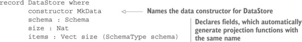
- There can be only one constructor.
- The fields give rise to projection functions, automatically generated from the types of the fields.
In the case of DataStore, you can see the types of the MkData data constructor and the projection functions generated from the fields by using :doc:
*DataStore> :doc DataStore Record DataStore Constructor: MkData : (schema : Schema) -> (size : Nat) -> (items : Vect size (SchemaType schema)) -> DataStore Projections: schema : (rec : DataStore) -> Schema size : (rec : DataStore) -> Nat items : (rec : DataStore) -> Vect (size rec) (SchemaType (schema rec))
You can try this by creating a simple test record at the REPL:
*DataStore> :let teststore = (MkData (SString .+. SInt) 1 [("Answer", 42)]) *DataStore> :t teststore teststore : DataStore Next, you can project the schema, the size, and the list of items from this test record:
*DataStore> schema teststore SString .+. SInt : Schema *DataStore> size teststore 1 : Nat *DataStore> items teststore [("Answer", 42)] : Vect 1 (String, Int) Records are actually much more flexible than can be seen in this small example. As well as projecting out the values of fields, Idris provides a syntax for setting fields and updating records. You’ll learn more about records when we discuss working with state in chapter 12.
6.3.3. Correcting compilation errors using holes
Now that you have a new definition of DataStore, your old program that uses it will no longer type-check because it relies on the old definition. The next step in refining your data store program, then, is to update the definitions so that the whole program
type-checks again. This doesn’t necessarily mean completing the program; at this stage, it’s fine to resolve type errors by inserting holes that you’ll fill in later.Earlier, I suggested temporarily commenting out the code after the definition of DataStore so that you could work on the refined definition without worrying about compilation errors. Now, we’ll work through the remainder of the program, uncommenting definitions bit by bit and repairing them, guided by the type errors Idris gives us.
First, let’s uncomment addToStore, defined previously as follows:
addToStore : DataStore -> String -> DataStore addToStore (MkData size store) newitem = MkData _ (addToData store) where addToData : Vect oldsize String -> Vect (S oldsize) String addToData [] = [newitem] addToData (item :: items) = item :: addToData items
On reloading, either by using Ctrl-Alt-R in Atom or the :r command at the REPL, Idris reports as follows:
DataStore.idr:21:1-11: When checking left hand side of addToStore: When checking an application of Main.addToStore: Type mismatch between Vect size (SchemaType schema) -> DataStore (Type of MkData schema size) and DataStore (Expected type)
The first problem here is that you’ve added an argument to MkData; it now requires a schema as well as a size and a vector of items. You can correct this by adding a schema argument to MkData:
addToStore : DataStore -> String -> DataStore addToStore (MkData schema size store) newitem = MkData schema _ (addToData store) where addToData : Vect oldsize String -> Vect (S oldsize) String addToData [] = [newitem] addToData (item :: items) = item :: addToData items
Idris now reports
Type mismatch between Vect size (SchemaType schema) (Type of store) and Vect size String (Expected type)
The problem is that the data store no longer stores merely Strings, but stores a type described by the schema. You can correct this by changing the types of addToStore and addToData so that they work with the correct type. A type-correct definition of addToStore is shown in the following listing.
Listing 6.12. A corrected definition of addToStore using the refined DataStore type
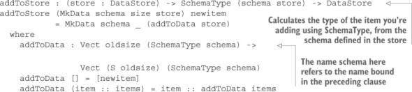
Listing 6.13. Old version of getEntry, with an error in the application of index
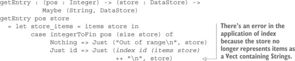
The problem is in the last line, where you extract an item from the store, because you’re treating the store as a Vect containing Strings. Here’s what Idris reports:
When checking an application of function Data.Vect.index: Type mismatch between Vect (size store) (SchemaType (schema store)) (Type of items store) and Vect (size store) String (Expected type)
The problem is in the application of index, which no longer returns a String. You can correct this error, temporarily, by inserting a hole to convert the result of index into a String, as follows.
Listing 6.14. Correcting getEntry by inserting a hole to convert the contents of the store to a displayable String
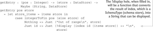
store : DataStore id : Fin (size store) pos : Integer store_items : Vect (size store) (SchemaType (schema store)) -------------------------------------- display : SchemaType (schema store) -> String
We’ll return to ?display shortly. For the moment, getEntry type-checks again. The next error is in processInput. Here’s the current definition.
Listing 6.15. Old version of processInput, with an error in the application of addToStore
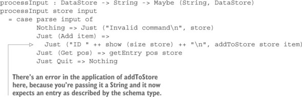
This definition has an error similar to getEntry, showing that you have a String but Idris expected a SchemaType (schema store):
When checking an application of function Main.addToStore: Type mismatch between String (Type of item) and SchemaType (schema store) (Expected type)
One possible fix is, as with getEntry, to add a hole for converting the String to an appropriate SchemaType (schema store) in processInput:
Just ("ID " ++ show (size store) ++ "\n", addToStore store (?convert item)) Alternatively, you could refine the definition of Command so that it only represents valid commands, meaning that any user input that’s invalid would lead to a parse error. We’ll take this approach, because it involves defining a more precise intermediate type, so you’ll check the validity of the input as early as possible.
To achieve this, parameterize Command by the schema description, and change the Add command so that it takes a SchemaType rather than the String input directly. Here’s the refined definition of Command.
Listing 6.16. Command, refined to be parameterized by the schema in the data store
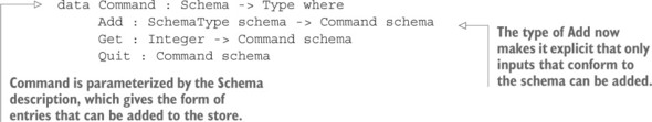
Listing 6.17. Updating parseCommand so that it parses inputs that conform to the schema
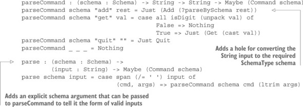
The resulting hole has a type that explains that it converts a String to an appropriate instance of the SchemaType schema:
schema : Schema rest : String -------------------------------------- parseBySchema : String -> SchemaType schema
There’s still a problem here, however! This function can’t be total because not every String is going to be parsable as a valid instance of the schema. Nevertheless, your goal at the moment is merely to make the overall program type-check again. We’ll return to this problem shortly.
You’ve refined the type of Command, added the schema argument to parse, and inserted holes for displaying entries (?display) and converting user input into entries (?parseBySchema). All that remains is to update processInput and main to use the new definitions. These are minor changes, shown in the next listing. In processInput, you pass the current schema to parse, and in main you set the initial schema to simply accept Strings.
Listing 6.18. Updated processInput and main, with a default schema
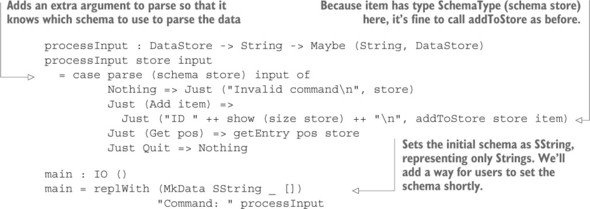
6.3.4. Displaying entries in the store
You now have two holes to fill in before you can execute this program. The first is ?display, which converts an entry in the store into a String, where the schema in the store gives the form of the data:
store : DataStore id : Fin (size store) pos : Integer store_items : Vect (size store) (SchemaType (schema store)) -------------------------------------- display : SchemaType (schema store) -> String
In this case, using Ctrl-Alt-L to lift the hole to a top-level function gives you a lot of information that you don’t need to implement display. All you really need is a schema description and the data.
Instead, you can implement display by hand as follows:
- Type— First, you can write a more generic type than Idris suggested. Rather than specifically using a schema extracted from a store, you can display data according to any schema:
display : SchemaType schema -> String
- Define— In order to define this function, you need to know about the schema itself. Otherwise, you won’t know what form the data is in. Add a skeleton definition, and then bring the implicit argument schema into scope:
display : SchemaType schema -> String display {schema} item = ?display_rhs - Define— You can define the function by case splitting on schema. Because the type of item is SchemaType schema, case splitting on schema will give you more information about the expected type of item:
display : SchemaType schema -> String display {schema = SString} item = ?display_rhs_1 display {schema = SInt} item = ?display_rhs_2 display {schema = (x .+. y)} item = ?display_rhs_3 - Type— Inspecting each of the resulting holes (?display_rhs_1, ?display_rhs_2 and ?display_rhs_3) tells you what item must be in each case:
item : String -------------------------------------- display_rhs_1 : String item : Int -------------------------------------- display_rhs_2 : String x : Schema y : Schema item : (SchemaType x, SchemaType y) -------------------------------------- display_rhs_3 : String
- Refine— For ?display_rhs_1 and ?display_rhs_2 you can complete the definition by directly converting item to a String. For ?display_rhs_3, you can case-split on item and recursively display each entry:
display : SchemaType schema -> String display {schema = SString} item = show item display {schema = SInt} item = show item display {schema = (x .+. y)} (iteml, itemr) = display iteml ++ ", " ++ display itemr
Once this definition is complete and the file is reloaded into the Idris REPL, there should be one remaining hole, ?parseBySchema.
6.3.5. Parsing entries according to the schema
The remaining hole, ?parseBySchema, is intended to convert the String the user entered into an appropriate type for the schema. You can see what’s expected by looking at its type:
rest : String schema : Schema -------------------------------------- parseBySchema : String -> SchemaType schema
As you saw earlier, not every String will lead to a valid SchemaType schema, so you can refine this type slightly and create a top-level function that returns a Maybe (SchemaType schema) to reflect the fact that parsing the input might fail, additionally making schema explicit:
parseBySchema : (schema : Schema) -> String -> Maybe (SchemaType schema)Then, you can edit parseCommand to use this new function. If parseBySchema fails (that is, returns Nothing), parseCommand should also return Nothing:
parseCommand schema "add" rest = case parseBySchema schema rest of Nothing => Nothing Just restok => Just (Add restok)
To parse complete inputs as described by schemas, you’ll need to be able to parse portions of the input according to a subset of the schema. For example, given a schema (SInt .+. SString) and an input 100 "Antelopes", you’ll need to be able to parse the prefix 100 as SInt, followed by the remainder, "Antelopes", as SString.
You can therefore define your parser with the following two components:
- parsePrefix reads a prefix of the input according to the schema and returns the parsed input, if successful, paired with the remainder of the text.
- parseBySchema calls parsePrefix with some input and ensures that once it has parsed the input according to the schema, there’s no input remaining.
The next listing shows the top-level implementation of parseBySchema and the type of the parsePrefix helper function.
Listing 6.19. Outline implementation of parseBySchema, using an undefined parsePrefix function to parse a prefix of an input according to a schema
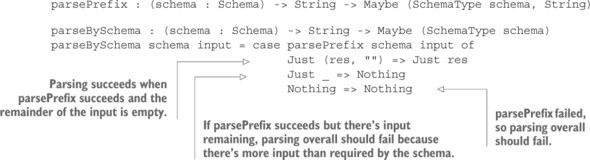
Let’s take a look at the outline of parsePrefix, following the type-define-refine approach and see how the structure of the schema gives us hints about how to proceed with each part of the implementation:
- Define— You already have the type, so begin by providing a skeleton definition:
parsePrefix : (schema : Schema) -> String -> Maybe (SchemaType schema, String) parsePrefix schema item = ?parsePrefix_rhs
- Define— If you case-split on schema, Idris will generate cases for each possible form of the schema:
parsePrefix : (schema : Schema) -> String -> Maybe (SchemaType schema, String) parsePrefix SString input = ?parsePrefix_rhs_1 parsePrefix SInt input = ?parsePrefix_rhs_2 parsePrefix (x .+. y) input = ?parsePrefix_rhs_3
- Type— Looking at the types of the holes tells you what the return types must be for each form of the schema. For example, in ?parsePrefix_rhs_2 you need to convert the input into a Int, if possible, paired with the rest of the input:
input : String -------------------------------------- parsePrefix_rhs_2 : Maybe (Int, String)
- Refine— For ?parsePrefix_rhs_2, if the prefix of the input contains digits, you can convert them to an Int and return the resulting Int and the remainder of the String. You can refine it to the following:
parsePrefix SInt input = case span isDigit input of ("", rest) => Nothing (num, rest) => Just (cast num, ltrim rest)If the prefix of the input that contains digits is empty, then it’s not a valid Int, so return Nothing. Otherwise, you can convert the prefix to an Int and return the rest of the input, with leading spaces trimmed using ltrim. - Refine— You can refine ?parsePrefix_rhs_1 similarly, looking for an opening quotation mark and then reading the string until you reach the closing quotation mark. You’ll see the complete definition shortly in listing 6.20.
- Refine— The type of ?parsePrefix_rhs_3 shows that you need to parse two subschemas and combine the results:
x : Schema y : Schema input : String -------------------------------------- parsePrefix_rhs_3 : Maybe ((SchemaType x, SchemaType y), String)
It’s a good idea to give x and y more-meaningful names before proceeding:parsePrefix (schemal .+. schemar) input = ?parsePrefix_rhs_3
To refine parsePrefix_rhs_3, you can recursively parse the first portion of the input according to schemal, and if that succeeds, parse the rest of the input according to schemar. Parse the first portion:parsePrefix (schemal .+. schemar) input = case parsePrefix schemal input of Nothing => Nothing Just (l_val, input') => ?parsePrefix_rhs_2
If parsePrefix on the first part of the schema fails, the whole thing will fail. Otherwise, you have a new hole:schemal : Schema l_val : SchemaType schemal input' : String schemar : Schema input : String -------------------------------------- parsePrefix_rhs_2 : Maybe ((SchemaType schemal, SchemaType schemar), String)
Keep reloading!
While following this type-driven approach, you always have a file that type-checks as far as possible. Here, rather than filling the hole completely, you’ve written a small part of it with a new hole, and checked that what you have type-checks before proceeding.
- Refine— Finally, you can complete this case by parsing the remaining input according to schemar:
parsePrefix (schemal .+. schemar) input = case parsePrefix schemal input of Nothing => Nothing Just (l_val, input') => case parsePrefix schemar input' of Nothing => Nothing Just (r_val, input'') => Just ((l_val, r_val), input'')
Nested case blocks
These nested case blocks we’ve used may seem a little verbose. In section 6.3.7 you’ll see one way of writing these more concisely.
The following listing shows the complete implementation of parsePrefix, filling in the remaining details, including parsing quoted strings. You now have a complete implementation that can compile and run.
Listing 6.20. Parsing a prefix of an input according to a specific schema
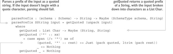
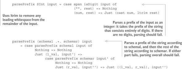
6.3.6. Updating the schema
Although you now have a complete implementation, it still has no more functionality than the previous version, because the schema is initialized as SString in main, and you haven’t yet implemented any way to update this:main : IO () main = replWith (MkData SString _ []) "Command: " processInput
You can, at least, try out different schemas by updating main and recompiling. For example, you could try a schema that accepts two Strings and an Int:
main : IO () main = replWith (MkData (SString .+. SString .+. SInt) _ []) "Command: " processInput
You can compile and run this using :exec at the REPL, and try a couple of example entries:
*DataStore> :exec Command: add "Bob Dylan" "Blonde on Blonde" 1965 ID 0 Command: add "Prefab Sprout" "From Langley Park to Memphis" 1988 ID 1 Command: get 0 "Bob Dylan", "Blonde on Blonde", 1965
It would be preferable, however, to allow users to define their own schemas, rather than hardcoding them into main. To achieve this, you can add a new command for setting a new schema, updating the Command data type.
Listing 6.21. The Command data structure with a new command for updating the schema
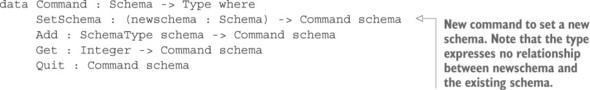
You’ll also need functions to do the following:
- Update the DataStore type to hold the new schema. This should only work when the store is empty, because when you change the schema type, it invalidates the current contents of the store.
- Parse a schema description from user input.
Listing 6.22. Parsing a Schema description, and extending the parser for Command to support setting a new schema
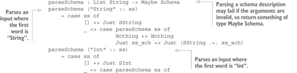
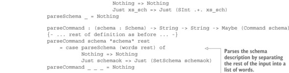
Listing 6.23 shows how updating the schema works once the new command has been parsed. As a design choice, it will only allow the schema to be updated when the store is empty, because there is no general way of updating the contents of the data store with an arbitrarily updated schema (an alternative would be to empty the store when the user changes the schema).
Listing 6.23. Processing the SetSchema command, updating the schema description in the DataStore
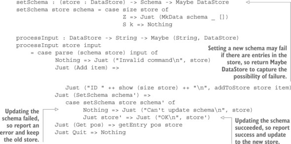
*DataStore> :exec Command: schema Int String OK Command: add 99 "Red balloons" ID 0 Command: add 76 "Trombones" ID 1 Command: schema String String Int Can't update schema when entries in store Command: get 1 76, "Trombones"
In the end, using a data type to describe the schema and using that schema to calculate the types of the operations on the data store has a few consequences:
- On reading user input, you can’t add the input to the store if it’s not valid according to the schema.
- If you change the schema type, you can’t invalidate the contents of the store because the type of the store’s contents prevents it. Changing the schema type requires you to have an empty store.
- When writing the parser for user input, you can use the description of the schema to guide the implementation of the parser and to build the correct type for the input.
6.3.7. Sequencing expressions with Maybe using do notation
In the data store program, there are several places where we’ve used a case block to check the result of a function that returns something with a Maybe type, and passed that result on. For example:
parseCommand schema "schema" rest = case parseSchema (words rest) of Nothing => Nothing Just schemaok => Just (SetSchema schemaok)
Here, parseCommand, which returns something of type Maybe (Command schema), has called parseSchema, which returns something of type Maybe Schema, and has used a case expression to check the result of the call to parseSchema.
If parseSchema fails, parseCommand also fails. Similarly, if parseSchema succeeds, then parseCommand also succeeds.You can see a similar pattern in the maybeAdd function in the following listing, which adds two values of type Maybe Int, returning Nothing if either input is Nothing.
Listing 6.24. Adding two Maybe Ints (Maybe.idr)
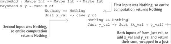
You can try maybeAdd on a few examples, and you’ll see that it adds its inputs if both are of the form Just val for some concrete value val, and that it returns Nothing if either of the inputs is Nothing:
*Maybe> maybeAdd (Just 3) (Just 4) Just 7 : Maybe Int *Maybe> maybeAdd (Just 3) Nothing Nothing : Maybe Int *Maybe> maybeAdd Nothing (Just 4) Nothing : Maybe Int
A common pattern is found here, in parseCommand, and in several other places throughout the data store implementation:
- Evaluate an expression of type Maybe ty. The result is either Nothing or Just x, where x has type ty.
- If the result is Nothing, the result of the entire computation is Nothing.
- If the result is Just x, pass x to the rest of the computation.
When you see a common pattern, it’s a good idea to try to capture that pattern in a higher-order function. In fact, you’ve already seen an operator that implements a similar pattern in chapter 5, when sequencing IO operations:
(>>=) : IO a -> (a -> IO b) -> IO b
The same operator works for sequencing Maybe computations, when defined as follows:
(>>=) : Maybe a -> (a -> Maybe b) -> Maybe b (>>=) Nothing next = Nothing (>>=) (Just x) next = next xEffectively, it takes the output of the first computation, if successful (that is, returning a Just), and passes it on as input to the second. It captures a common pattern of evaluating an expression with a Maybe type.
Remember from chapter 5 that if you check the type of (>>=) at the REPL, you’ll see a constrained generic type:
Idris> :t (>>=) (>>=) : Monad m => m a -> (a -> m b) -> m b
In general, the >>= operator can be used to sequence computations. You’ll see how this works in chapter 7 when we discuss interfaces.
Using (>>=) as an infix operator, you can rewrite maybeAdd more concisely, if somewhat cryptically, as in the following listing.
Listing 6.25. Adding two Maybe Ints using (>>=) rather than direct case analysis
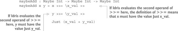
In chapter 5, you saw that Idris provides a special notation for sequencing computations using (>>=), introduced by the keyword do. You can use the same notation here, and write maybeAdd as follows.
Listing 6.26. Adding two Maybe Ints using do notation rather than using (>>=) directly
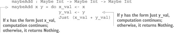
Figure 6.5 shows how an expression using do notation is translated into an expression using (>>=). This works exactly the same way as the translation of IO programs written using do notation. Just like the translation of list syntax into Nil and (::), this translation is purely syntactic. As a result, if you define the (>>=) operator in some other context, Idris will allow you to use do notation in that context.
Figure 6.5. Transforming do notation to an expression using the (>>=) operator
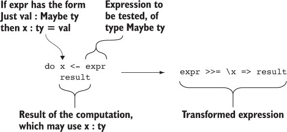
parseCommand schema "schema" rest = do schemaok <- parseSchema (words rest) Just (SetSchema schemaok)
Exercises
- Update the data store program to support Chars in the schema. You can test your solution at the REPL as follows:
*ex_6_3> :exec Command: schema Char Int OK Command: add x 24 ID 0 Command: add y 17 ID 1 Command: get 0 'x', 24
- Modify the get command so that, if given no arguments, it prints the entire contents of the data store. For example:
*ex_6_3> :exec Command: schema Char Int OK Command: add x 24 ID 0 Command: add y 17 ID 1 Command: get 0: 'x', 24 1: 'y', 17
- Update the data store program so that it uses do notation rather than nested case blocks, where appropriate.
6.4. Summary
- Type synonyms are alternative names for existing types, which allow you to give more-descriptive names to types.
- Type-level functions are functions that can be used anywhere that Idris is expecting a Type. Type synonyms are a special case of type-level functions.
- Type-level functions can be used to compute types, and they allow you to write functions with varying numbers of arguments, such as printf.
- You can represent a schema for a data store as a type, and then use type-level functions to calculate the types of operations, such as parsing and displaying entries in the data store from the schema description.
- A record is a data type with only one constructor, and with automatically generated functions for projecting fields from the record.
- After refining a data type, you can use holes to correct compilation errors temporarily.
- Using do notation, you can sequence computations that use Maybe to capture the possibility of errors.
Chapter 7. Interfaces: using constrained generic types
This chapter covers- Constraining generic types using interfaces
- Implementing interfaces for specific contexts
- Using interfaces defined in the Prelude
In chapter 2, you saw that generic function types with type variables could be constrained so that the variables stood for a more limited set of types. For example, you saw the following function for doubling a number in any numeric type:
double : Num a => a -> a double x = x + x
The type of double includes a constraint, Num a, which states that a can only stand for numeric types. Therefore, you can use double with Int, Nat, Integer, or any other numeric type, but if you try to use it with a non-numeric type, such as Bool, Idris will report an error.
You’ve seen a few such constraints, such as Eq for types that support equality tests and Ord for types that support comparisons. You’ve also seen functions that
rely on other constraints that we haven’t discussed in detail, such as map and >>=, which rely on Functor and Monad, respectively. We haven’t yet discussed how these constraints are defined or introduced.In this chapter, we’ll discuss how to define and use constrained generic types using interfaces. In the type declaration for double, for example, the constraint Num a is implemented by an interface, Num, which describes arithmetic operations that will be implemented in different ways for different numeric types.
Type classes in Haskell
If you know Haskell, you’ll be familiar with Haskell’s concept of type classes. Interfaces in Idris are similar to type classes in Haskell and are often used in the same way, though there are some differences. The most important are, first, that interfaces in Idris can be parameterized by values of any type, and are not limited to types or type constructors, and, second, interfaces in Idris can have multiple implementations, though we won’t go into the details in this chapter.
From the perspective of type-driven development, interfaces allow us to give the necessary level of precision to generic types. In general, an interface in Idris describes a collection of generic operations that can be implemented in different ways for different concrete types. For example:
- You could define an interface for operations that serialize and load generic data to and from JSON.
- A graphics library could provide an interface for operations that draw representations of data.
The Prelude includes a wide range of interfaces, and we’ll concentrate on these in this chapter. We’ll begin by looking in detail at two of the most important.
7.1. Generic comparisons with Eq and Ord
To begin, we’ll look at two interfaces that define generic comparisons, both of which are defined in the Prelude:
- Eq, which supports comparing values for equality or inequality.
- Ord, which supports comparing values to determine which is larger.
In doing so, you’ll learn how to declare interfaces, how to implement those interfaces in specific contexts, and how different interfaces can relate to each other.
7.1.1. Testing for equality with Eq
As you saw in chapter 2, Idris provides an operator for testing values for equality, ==, with a constrained generic type:
Idris> :t (==) (==) : Eq ty => ty -> ty -> BoolIn other words, you can compare two values of some generic type ty for equality, returning a result as a Bool, provided that ty satisfies the Eq constraint. Similarly, there’s an operator for testing for inequality:
Idris> :t (/=) (/=) : Eq ty => ty -> ty -> Bool
In the example in this section, I’ve specified exactly one constraint, Eq ty. You can also list multiple constraints as a comma-separated list. For example, the following function type specifies that ty needs to satisfy the Num and Show constraints:
addAndShow : (Num ty, Show ty) => ty -> ty -> String
You’ll see more examples later, in section 7.2.2.
Any time you use either of these operators, you must know that its operands are of a type that can be compared for equality. Let’s say, for example, you want to write a function that counts the number of occurrences of a specific value, of some generic type ty, in a list. We’ll create a function called occurrences in a file, Eq.idr:
- Type— As always, begin by giving a type for the function and creating a skeleton definition:
occurrences : (item : ty) -> (values : List ty) -> Nat occurrences item xs = ?occurrences_rhs
- Define, refine— You can define the function by case splitting on the input list, xs, and refining the hole generated in each case. If it’s an empty list, there can be no occurrences of item, so return 0:
occurrences : (item : ty) -> (values : List ty) -> Nat occurrences item [] = 0 occurrences item (value :: values) = ?occurrences_rhs_2
- Refine— If the input is a non-empty list, try testing the value at the start of the list and item for equality:
occurrences : (item : ty) -> (values : List ty) -> Nat occurrences item [] = 0 occurrences item (value :: values) = case value == item of case_val => ?occurrences_rhs_2
Unfortunately, Idris reports an error:Eq.idr:3:13: When checking right hand side of occurrences with expected type Nat Can't find implementation for Eq ty
This problem is similar to the one we encountered in chapter 3 when defining ins_sort. In this case, value and item have type ty, but there’s no constraint that values of type ty are comparable for equality. - Refine— The solution, as with ins_sort, is to refine the type by adding a constraint:
occurrences : Eq ty => (item : ty) -> (values : List ty) -> Nat
The constraint Eq ty means that you can now use the == operator and complete the definition as follows:occurrences : Eq ty => (item : ty) -> (values : List ty) -> Nat occurrences item [] = 0 occurrences item (value :: values) = case value == item of False => occurrences item values True => 1 + occurrences item values
The final type of occurrences says that it takes a ty and a List ty as inputs, provided that the type variable ty stands for a type that can be compared for equality.
This works fine for built-in types such as Char and Integer:
*Eq> occurrences 'b' ['a','a','b','b','b','c'] 3 : Nat *Eq> occurrences 100 [50,100,100,150] 2 : Nat
But what if you have user-defined types? Let’s say you have a user-defined type named Matter, also defined in Eq.idr:
data Matter = Solid | Liquid | Gas
You’d hope to be able to count the number of occurrences of Liquid in a list. Unfortunately, if you try this, Idris reports an error:
*Eq> occurrences Liquid [Solid, Liquid, Liquid, Gas] Can't find implementation for Eq Matter
This error message means that Idris doesn’t know how to compare values in the user-defined Matter type for equality. To correct this, we’ll need to take a look at how the Eq constraint is defined, and how to explain to Idris how user-defined types such as Matter can satisfy it.
7.1.2. Defining the Eq constraint using interfaces and implementations
Constraints such as Eq are defined in Idris using interfaces. An interface definition contains a collection of related functions (called methods of the interface) that can be given different implementations for specific contexts. The Eq interface is defined in the Prelude, containing the methods (==) and (/=).
Listing 7.1. The Eq interface (defined in the Prelude)
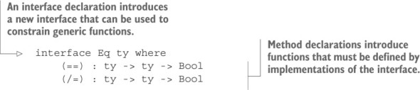
(==) : Eq ty => ty -> ty -> Bool (/=) : Eq ty => ty -> ty -> Bool
Figure 7.1 shows the components of the interface declaration. The parameter, ty in this case, is assumed to have type Type by default, and stands for the generic argument that’s to be constrained. The parameter must appear in each of the method declarations.
Figure 7.1. The Eq interface declaration
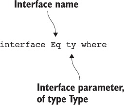
Parameter naming conventions
The parameters of an interface (ty here) are typically generic type variables, so I typically give them short, generic, names. The name ty indicates that the parameter could be any type. When there are more parameters, or where the interface has a more specific purpose, I give more-specific names.
An interface declaration, then, provides the types for related functions with a parameter standing for a generic argument. To define these functions for specific cases, you need to provide implementations.
To write an implementation, you give the interface and a parameter, along with definitions for each of the methods. The following listing shows an implementation for the Eq interface, which explains how the Matter type satisfies the constraint.
Listing 7.2. Implementation of Eq for Matter (Eq.idr)
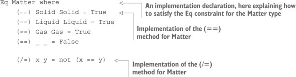
Interactive development of implementations
As you’ll see shortly, you can use Ctrl-Alt-A to provide a skeleton implementation of Eq Matter, as with function definitions.
If you add this implementation to the file in which you defined occurrences and Matter, you’ll now be able to use occurrences with a List Matter:
*Eq> occurrences Liquid [Solid, Liquid, Liquid, Gas] 2 : Nat
This provides implementations of the two methods, (==) and (/=), which are required to be implemented in order to be able to compare elements of type Matter for equality and inequality. Note that the implementation doesn’t contain any type declarations, because these are given in the interface declaration.
If you use :doc on an interface at the REPL, or Ctrl-Alt-D over an interface name in Atom, Idris will show documentation for the interface including its parameters, methods, and a list of the known implementations. For example, here’s what it looks like for Eq:
Idris> :doc Eq Interface Eq The Eq interface defines inequality and equality. Parameters: ty Methods: (==) : Eq ty => ty -> ty -> Bool infixl 5 The function is Total (/=) : Eq ty => ty -> ty -> Bool infixl 5 The function is Total Implementations: Eq () Eq Int Eq Integer Eq Double [...]
You can build the implementation interactively in Atom as follows:
- Type— Start by giving the implementation header on its own:
Eq Matter where
This a Type step because it instantiates the types of (==) and (/=), with Matter standing for the parameter a. - Define— You can also use the interactive editing tools in Atom to build implementations of interfaces. With the cursor over Eq, press Ctrl-Alt-A, and Idris will add skeleton definitions for (==) and (/=) with generic names for the arguments:
Eq Matter where (==) x y = ?Eq_rhs_1 (/=) x y = ?Eq_rhs_2
- Type— If you check the type of ?Eq_rhs_1, you’ll see confirmation that x and y are of type Matter:
x : Matter y : Matter -------------------------------------- Eq_rhs_1 : Bool
- Define— You can begin by defining (==) by case splitting on x:
Eq Matter where (==) Solid y = ?Eq_rhs_3 (==) Liquid y = ?Eq_rhs_4 (==) Gas y = ?Eq_rhs_5 (/=) x y = ?Eq_rhs_2
- Refine— Each value of type Matter is only equal to itself, so you can refine the definition as follows, with a catchall case to handle when the inputs aren’t equal:
Eq Matter where (==) Solid Solid = True (==) Liquid Liquid = True (==) Gas Gas = True (==) _ _ = False (/=) x y = ?Eq_rhs_2
Remember that the order of cases is important, and Idris will try to match the clauses in order, so the catchall case must be at the end. - Refine— To complete the implementation, you need to define (/=). The simplest definition is to use (==) and then invert the result:
Eq Matter where (==) Solid Solid = True (==) Liquid Liquid = True (==) Gas Gas = True (==) _ _ = False (/=) x y = not (x == y)
7.1.3. Default method definitions
Interfaces define a collection of related methods, such as (==) and (/=). In some cases, methods are so closely related that you can define them in terms of other methods in the interface. For example, you’d always expect the result of x /= y to be the opposite of the result of x == y, no matter what the values or even types of x and y.
For this situation, Idris allows you to provide a default definition for a method. If an implementation doesn’t provide a definition for a method that has a default definition, Idris uses that default. For example, the Eq interface provides defaults for both (==) and (/=), each defined in terms of the other, as follows.
Listing 7.3. Eq interface with default method definitions
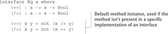
You can therefore provide an implementation of Eq for Matter by providing only a definition of (==), and using the default method implementation for (/=):
Eq Matter where (==) Solid Solid = True (==) Liquid Liquid = True (==) Gas Gas = True (==) _ _ = False
The default method definitions mean that when you’re defining an implementation of Eq, you can provide definitions for either or both of (==) and (/=).
7.1.4. Constrained implementations
When writing implementations for generic types, you may discover the need for additional constraints on the parameters of the generic types. For example, to check whether two lists are equal, you’ll need to know how to compare the element types for equality.
In chapter 4, you saw the generic type of binary trees, defined as follows in tree.idr:
data Tree elem = Empty | Node (Tree elem) elem (Tree elem)To check whether two trees are equal, you’ll also need to be able to compare the element types. Let’s see what happens if you try to define an implementation of Eq for Trees with a generic element type:
- Type— Begin by writing the implementation header, stating the interface you wish to implement and the type for which you’re implementing it:
Eq (Tree elem) where
- Define— Add a skeleton definition that gives template definitions for all the methods of the interface:
Eq (Tree elem) where (==) x y = ?Eq_rhs_1 (/=) x y = ?Eq_rhs_2
You can use the default definition for (/=), so you can delete the second method:Eq (Tree elem) where (==) x y = ?Eq_rhs_1
- Define— As with the Eq implementation for Matter, you can define (==) by case splitting on each argument and using a catchall case for cases where the inputs are unequal. You know that Empty equals itself, Nodes are equal if all their arguments are equal, and everything else is not equal:
Eq (Tree elem) where (==) Empty Empty = True (==) (Node left e right) (Node left' e' right') = ?Eq_rhs_3 (==) _ _ = False
For the moment, you’ve left a hole, ?Eq_rhs_3, for the details of comparing Nodes. - Refine— You’d expect to be able to complete the definition by refining the ?Eq_rhs_3 hole to say that you can compare each corresponding argument:
Eq (Tree elem) where (==) Empty Empty = True (==) (Node left e right) (Node left' e' right') = left == left' && e == e' && right == right' (==) _ _ = False
But, unfortunately, Idris reports a problem:Can't find implementation for Eq elem
You can compare left and left' for equality, and correspondingly right and right', because they’re of type Tree elem, and the implementation can be recursive; you’re currently defining equality for Tree elem. But e and e' are of type elem, a generic type, and you don’t necessarily know how to compare elem for equality. - Refine— The solution is to refine the implementation declaration by constraining it to require that elem also has an implementation of Eq available:
Eq elem => Eq (Tree elem) where (==) Empty Empty = True (==) (Node left e right) (Node left' e' right') = left == left' && e == e' && right == right' (==) _ _ = False
The constraint appears to the left of the arrow, =>, the same way as constraints appear in type declarations. Figure 7.2 shows the components of this interface header.
Figure 7.2. Constrained implementation header
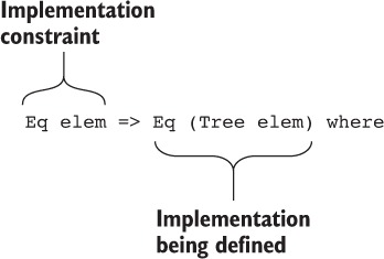
You can read this header as stating that generic trees can be compared for equality, provided that their element type can also be compared for equality. You can introduce interface constraints like this anywhere you introduce a type variable, if you need to constrain that type variable further.
Limitations on implementation parameters
You’ve now seen implementations of Eq parameterized by Matter and by Tree elem, both of which are of type Type. But you can’t parameterize implementations by everything of type Type. You’re limited to names introduced by either a data or record declaration, or primitive types. In particular, this means you can’t parameterize implementations by type synonyms or functions that compute types.
You’ve already seen constraints on type declarations, and here you’ve seen one in an implementation definition. In the same way, you can place constraints on interface definitions themselves.
7.1.5. Constrained interfaces: defining orderings with Ord
If you place a constraint on an interface definition, you’re effectively extending an existing interface. In the Prelude, for example, there’s an Ord interface, shown in the next listing, that extends Eq to support ordering of values.
Listing 7.4. The Ord Interface, which extends Eq (defined in the Prelude)
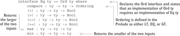
All methods, except compare, have default definitions, some of which are written in terms of compare, and some of which use the (==) method provided by the Eq interface.
If you have an implementation of Ord for some data type, you can sort lists containing that type:
sort : Ord ty => List ty -> List ty
For example, you might have a data type representing a music collection, with records containing a title, artist, and year of release, and you may wish to sort them first by artist name, then by year of release, and then by title. The following listing gives a definition of this data type with some examples.
Listing 7.5. A record data type and a collection to be sorted (Ord.idr)
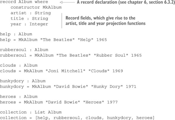
If you try sorting the collection as it stands, Idris will report that it doesn’t know how to order values of type Album:
*Ord> sort collection Can't find implementation for Ord Album
Listing 7.6 shows how you can explain to Idris how to order Albums. First, you need to give an Eq implementation, because the constraint on the Ord interface requires that implementations of Ord are also implementations of Eq. The Eq implementation checks that each field has the same value; the Ord implementation compares by artist name, and then by year, and then by title if the first two are equal.
Listing 7.6. Implementations of Eq and Ord for Album
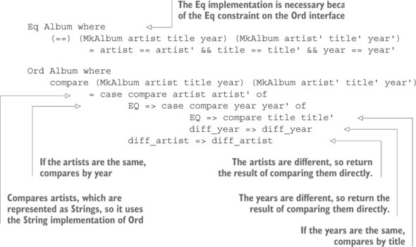
*Ord> heroes > clouds False : Bool *Ord> help <= rubbersoul True : Bool
It also means that you can use any function with an Ord constraint, such as sort. For example, you can sort the collection and list the titles in sorted order:
*Ord> map title (sort collection) ["Hunky Dory", "Heroes", "Clouds", "Help", "Rubber Soul"] : List String
Giving constraints on interfaces, like the Eq constraint on Ord, allows you to define hierarchies of interfaces. So, for example, if there’s an implementation of Ord for some type, you know it’s safe to assume that there’s also an implementation of Eq for that type. The Prelude defines several interfaces, some arranged into hierarchies, and we’ll look at some of the most important in the next section.
Exercises
For these exercises, you’ll use the Shape type defined in chapter 4:
data Shape = Triangle Double Double | Rectangle Double Double | Circle Double
- Implement Eq for Shape. You can test your answer at the REPL as follows:
*ex_7_1> Circle 4 == Circle 4 True : Bool *ex_7_1> Circle 4 == Circle 5 False : Bool *ex_7_1> Circle 4 == Triangle 3 2 False : Bool
- Implement Ord for Shape. Shapes should be ordered by area, so that shapes with a larger area are considered greater than shapes with a smaller area. You can test this by trying to sort the following list of Shapes:
testShapes : List Shape testShapes = [Circle 3, Triangle 3 9, Rectangle 2 6, Circle 4, Rectangle 2 7]
You should see the following when sorting the list at the REPL:*ex_7_1> sort testShapes [Rectangle 2.0 6.0, Triangle 3.0 9.0, Rectangle 2.0 7.0, Circle 3.0, Circle 4.0] : List Shape
7.2. Interfaces defined in the Prelude
The Idris Prelude provides several commonly used interfaces, in addition to Eq and Ord, as you’ve just seen. In this section and the next, I’ll briefly describe some of the most important. We’ve encountered several in passing already: Show, Num, Cast, Functor, and Monad. Here, you’ll see how these interfaces are defined, where they might be used, and some examples of how you can write implementations of them for your own types.
The parameters of an interface (in other words, the variables given in the interface header) can have any type. If there’s no explicit type given in the interface header for a parameter, it’s assumed to be of type Type. In this section, we’ll look at some interfaces that are parameterized by Types.
7.2.1. Converting to String with Show
In chapter 2, you saw the show function, which converts a value to a String. This is a method of the Show interface, defined in the Prelude and shown in the following listing. Both the show and showPrec methods have default implementations, each defined in terms of the other. Here, we’ll only consider show.
Listing 7.7. The Show interface (defined in the Prelude)
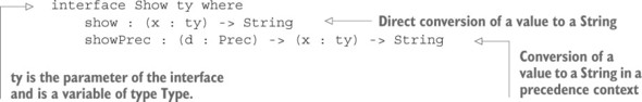
Precedence contexts
The purpose of showPrec is to be able to display complex expressions in parentheses if necessary. This might be useful if, say, you have a representation of arithmetic formulae, where precedence rules say that some subexpressions need to be parenthesized. By default, showPrec calls show directly, and for most display purposes this is entirely adequate. If you wish to investigate further, take a look at the documentation using :doc.The Prelude provides two functions that use show to convert a value to a String and then output it to the console, with or without a trailing newline character:
printLn : Show ty => ty -> IO () print : Show ty => ty -> IO ()
You can define a simple Show implementation for the Album type:
Show Album where show (MkAlbum artist title year) = title ++ " by " ++ artist ++ " (released " ++ show year ++ ")"
Then, you can print an Album to the console using printLn. For example:
*Ord> :exec printLn hunkydory Hunky Dory by David Bowie (released 1971)
The Show interface is primarily used for debugging output, to display values of complex data types in a human-readable form.
7.2.2. Defining numeric types
The Prelude provides a hierarchy of interfaces with methods for numeric operations. These interfaces divide operators into several groups:
- The Num interface—Contains operations that work on all numeric types, including addition, multiplication, and conversion from integer literals
- The Neg interface—Contains operations that work on numeric types that can be negative, including negation, subtraction, and absolute value
- The Integral interface—Contains operations that work on integer types
- The Fractional interface—Contains operations that work on numeric types that can be divided into fractions
The following listing shows how these interfaces are defined.
Listing 7.8. The numeric interface hierarchy (defined in the Prelude)
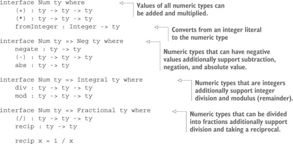
Table 7.1. Summary of numeric interfaces and their implementations
| Interface | Description | Implementations |
|---|---|---|
| Num | All numeric types | Integer, Int, Nat, Double |
| Neg | Numeric types that can be negative | Integer, Int, Double |
| Integral | Integer types | Integer, Int, Nat |
| Fractional | Numeric types that can be divided into fractions | Double |
One method that’s particularly worth noting is fromInteger. All integer literals in Idris are implicitly converted to the appropriate numeric type using fromInteger. As a result, as long as there’s an implementation of Num for a numeric type, you can use integer literals for that type.
By making new implementations of Num and related interfaces, you can use standard arithmetic notation and integer literals for your own types. For example, listing 7.9 shows an Expr data type that represents arithmetic expressions, including an “absolute value” operation and an eval function that calculates the result of evaluating an expression.
Listing 7.9. An arithmetic expression data type and an evaluator (Expr.idr)
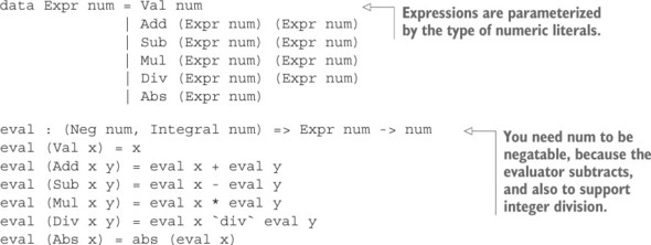
*Expr> Add (Val 6) (Mul (Val 3) (Val 12)) Add (Val 6) (Mul (Val 3) (Val 12)) : Expr Integer *Expr> eval (Add (Val 6) (Mul (Val 3) (Val 12))) 42 : Integer
If, on the other hand, you make a Num implementation for Expr, you’ll be able to use standard arithmetic notation (with +, *, and integer literals) to build values of type Expr. If, furthermore, you make a Neg implementation, you’ll be able to use negative numbers and subtraction. The following listing shows how you can do this.
Listing 7.10. Implementations of Num and Neg for Expr (Expr.idr)
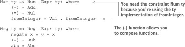
The (.) function gives you a concise notation for composing two functions. It has the following type and definition:
(.) : (b -> c) -> (a -> b) -> a -> c (.) func_bc func_ab x = func_bc (func_ab x)
In the example in listing 7.10, you could have written this:
fromInteger x = Val (fromInteger x)
The (.) function allows you instead to write this:
fromInteger x = (Val . fromInteger) xFinally, rather than have the x as an argument on both sides, you can use partial application:
fromInteger = Val . fromInteger
To construct an expression and evaluate it, you can use standard notation:
*Expr> the (Expr _) (6 + 3 * 12) Add (Val 6) (Mul (Val 3) (Val 12)) : Expr Integer *Expr> eval (6 + 3 * 12) 42 : Integer
In the first case, you need to use the to make it clear that the numeric expression should be interpreted as an Expr, rather than the default, which would be an Integer. In the second case, Idris infers from the type of eval that the argument must be an Expr.
7.2.3. Converting between types with Cast
In chapter 2, you saw the cast function, which is used to convert values between different, compatible types. If you look at the type of cast, you’ll see that it has a constrained generic type that uses a Cast interface:
Idris> :t cast cast : Cast from to => from -> to
Unlike the interfaces we’ve seen so far, Cast has two parameters rather than one. The next listing gives its definition. Interfaces in Idris can have any number of parameters (even zero!).
Listing 7.11. The Cast interface (defined in the Prelude)

As we observed in chapter 2, conversions using cast may be lossy. Idris defines casts between Double and Integer, for example, which may lose precision. The purpose of cast is to provide a convenient generic function, with an easy-to-remember name, for conversions.
To define an implementation of an interface with more than one parameter, you need to give both concrete parameters. For example, you could define a cast from Maybe elem to List elem, because you can think of Maybe elem as being a list of either zero or one elems:
Cast (Maybe elem) (List elem) where cast Nothing = [] cast (Just x) = [x]You could also define a cast in the other direction, from List elem to Maybe elem, but this would potentially lose information, because you’d need to decide which element to take if the list had more than one element.
Exercises
- Implement Show for the Expr type defined in section 7.2.2. Hint: To keep this simple and avoid concerns about precedence, assume all subexpressions can be written in parentheses. You can test your answer at the REPL as follows:
*ex_7_2> show (the (Expr _) (6 + 3 * 12)) "(6 + (3 * 12))" : String *ex_7_2> show (the (Expr _) (6 * 3 + 12)) "((6 * 3) + 12)" : String
- Implement Eq for the Expr type. Expressions should be considered equal if their evaluation is equal. So, for example, you should see the following:
*Expr> the (Expr _) (2 + 4) == 3 + 3 True : Bool *Expr> the (Expr _) (2 + 4) == 3 + 4 False : Bool
Hint: Start with the implementation header Eq (Expr ty) where, and add constraints as you discover you need them. - Implement Cast to allow conversions from Expr num to any appropriately constrained type num. Hint: You’ll need to evaluate the expression, which should tell you how num needs to be constrained. You can test your answer at the REPL as follows:
*ex_7_2> let x : Expr Integer = 6 * 3 + 12 in the Integer (cast x) 30 : Integer
7.3. Interfaces parameterized by Type -> Type
In all the interfaces we’ve seen so far, the parameters have been Types. There is, however, no restriction on what the types of the parameters can be. In particular, it’s common for interfaces to have parameters of Type -> Type. For example, you’ve already seen the following functions with constrained types:
map : Functor f => (a -> b) -> f a -> f b pure : Applicative f => a -> f a (>>=) : Monad m => m a -> (a -> m b) -> m b
In each case, the parameter f or m stands for a parameterized type, such as List or IO. You’ve seen map in the context of List, and pure and (>>=) in the context of IO.
In this section, we’ll look at how these and other operations are defined generically in the Prelude using interfaces, along with some examples of how to apply them to your own types.7.3.1. Applying a function across a structure with Functor
In chapter 2 you saw the map function, which applies a function to every element in a list:
Idris> map (*2) [1,2,3,4] [2, 4, 6, 8] : List Integer
I noted, however, that map isn’t limited to lists, but rather has a constrained generic type using the Functor interface. Functors allow you to apply a function uniformly across a generic type. The preceding example applied the “multiply by two” function uniformly across a list of Integers.
The following listing shows the definition of the Functor interface, which contains map as its only method, and its implementation for List, as defined in the Prelude.
Listing 7.12. The Functor interface and an implementation for List (defined in the Prelude)
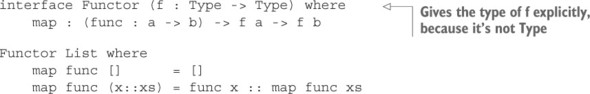
So far, the interfaces we’ve seen have been parameterized by a variable with type Type. But the parameter of Functor is itself a parameterized type (such as List). When the parameter has any type other than Type, you need to give the parameter’s type explicitly.
It’s often useful to provide an implementation of Functor for collection data structures. For example, the following listing shows how to define a Functor implementation for binary trees, uniformly applying a function across every element that appears at a Node.
Listing 7.13. Implementation of Functor for Tree (Tree.idr)
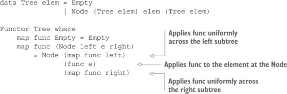
Listing 7.14. Implementation of Functor for vectors (defined in Data.Vect)

The parameter in the implementation’s header, Vect n, means that you’re defining an implementation of Functor for vectors of any length. The usual rules for implicit arguments apply, as described in chapter 3: any name beginning with a lowercase letter in a function argument position is treated as an implicit argument. Therefore, n is treated as an implicit argument here.
7.3.2. Reducing a structure using Foldable
If you write down a list of numbers in the form 1 :: 2 :: 3 :: 4 :: [], you can compute the sum of the numbers by applying the following rules:
- Replace each :: with a + (giving 1 + 2 + 3 + 4 + []).
- Replace the [] with a 0 (giving 1 + 2 + 3 + 4 + 0).
- Calculate the value of the resulting expression (giving 10).
Or you can compute the product of the numbers by applying the following rules:
- Replace each :: with a * (giving 1 * 2 * 3 * 4 * []).
- Replace the [] with a 1 (giving 1 * 2 * 3 * 4 * 1).
- Calculate the value of the resulting expression (giving 24).
In general, we’re reducing the contents of the list to a single value by replacing the [] with a default, or initial, value, and replacing :: with a function of two arguments, which combines each value with the result of reducing the rest of the list. Idris provides two higher-order functions, called folds to suggest folding the structure into a single value, to do exactly this:
foldr : (elem -> acc -> acc) -> acc -> List elem -> acc foldl : (acc -> elem -> acc) -> acc -> List elem -> acc
The distinction between foldr and foldl is in how the resulting expression is bracketed. In our first example, foldr would calculate the result as 1 + (2 + (3 + (4 + 0))), whereas foldl would calculate the result as (((0 + 1) + 2) + 3) + 4. In other words, foldr processes the elements left to right, and foldl processes the elements right to left.
Type variables in foldl and foldr
The names of the variables in the types of foldl and foldr suggest their purpose: elem is the element type of the list and acc is the type of the result. The name acc suggests the type of an accumulating parameter, in which the eventual result is computed.
In each case, the first argument is the function (or operator) to apply, and the second argument is the initial value. So, you can calculate the two previous examples as follows:
Idris> foldr (+) 0 [1,2,3,4] 10 : Integer Idris> foldr (*) 1 [1,2,3,4] 24 : Integer
Or you could use a fold to calculate the total length of the Strings in a List String. For example, the total length of ["One", "Two", "Three"] should be 11.
Let’s write this interactively, using foldr, in a file named Fold.idr:
- Type, define—You can begin with a type and a candidate definition, and apply foldr to the input list, xs, but leave holes for the function and initial value so their types can give you hints as to how to proceed:
totalLen : List String -> Nat totalLen xs = foldr ?sumLength ?initial xs
- Type, refine—The type of ?initial tells you that the initial value must be a Nat:
xs : List String t : Type -> Type elem : Type -------------------------------------- initial : Nat
You can initialize it with 0, because the total length of an empty list of strings is 0:totalLen : List String -> Nat totalLen xs = foldr ?sumLength 0 xs
- Type, refine—The type and context of ?sumLength tells you that you need to provide a function:
xs : List String t : Type -> Type elem : Type -------------------------------------- sumLength : String -> Nat -> Nat
The function you need to provide takes a String (standing for the string at a given position in the list) and a Nat (standing for the result of folding the rest of the list), and returns a Nat (standing for the total length). You can complete the definition as follows:totalLen : List String -> Nat totalLen xs = foldr (\str, len => length str + len) 0 xs
You can test the resulting function at the REPL:
*Fold> totalLen ["One", "Two", "Three"] 11 : NatIn the preceding example, I gave a type for foldr that was specific to List. But if you look at the type at the REPL, you’ll see a constrained generic type using a Foldable interface:
foldr : Foldable t => (elem -> acc -> acc) -> acc -> t elem -> acc
An implementation of Foldable for a structure explains how to reduce that structure to a single value using an initial value and a function to combine each element with an overall folded structure. The following listing gives the interface definition. There’s a default definition for foldl, written in terms of foldr, so only foldr need be implemented.
Listing 7.15. The Foldable interface (defined in the Prelude)
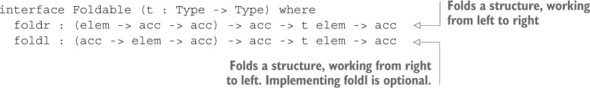
The next listing shows how Foldable is implemented in the Prelude for List. Note in particular the distinction between the implementations of foldr and foldl.
Listing 7.16. Implementation of Foldable for List (defined in the Prelude)
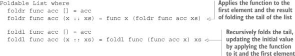
Because our Tree data type is a generic type containing a collection of values, you should be able to provide a Foldable implementation:
- Type— Begin by providing an implementation header and a skeleton definition of foldr. You can use the default definition for foldl:
Foldable Tree where foldr func acc tree = ?Foldable_rhs_1
- Define, refine—Case-split on the tree. If the tree is Empty, you return the initial value:
Foldable Tree where foldr func acc Empty = acc foldr func acc (Node left e right) = ?Foldable_rhs_3
- Refine— In the Node case, because foldr works left to right, you begin by folding the left subtree recursively. Figure 7.3 illustrates this with an example, assuming an initial accumulator of 0.
Figure 7.3. Fold the left subtree with the initial accumulator. This gives you 0 + 1 + 2 + 3 = 6.
In code, it looks like this: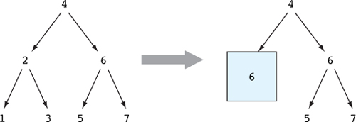
Foldable Tree where foldr func acc Empty = acc foldr func acc (Node left e right) = let leftfold = foldr func acc left in ?Foldable_rhs_3
- Refine— Next, take the result of folding the left subtree (leftfold) and use it as the initial value when folding the right subtree. Figure 7.4 illustrates this on the same example.
Figure 7.4. Fold the right subtree, initialized with the result of folding the left subtree. This gives you 6 + 5 + 6 + 7 = 24.
In code, it looks like this: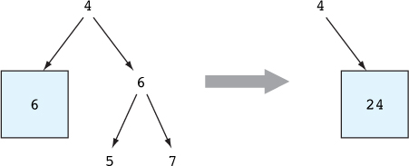
Foldable Tree where foldr func acc Empty = acc foldr func acc (Node left e right) = let leftfold = foldr func acc left rightfold = foldr func leftfold right in ?Foldable_rhs_3
- Refine— Finally, apply func to the value at the node e and the result of folding the right subtree:
Foldable Tree where foldr func acc Empty = acc foldr func acc (Node left e right) = let leftfold = foldr func acc left rightfold = foldr func leftfold right in func e rightfold
In the example, this gives you the result 4 + 24 = 28.
7.3.3. Generic do notation using Monad and Applicative
There are two other interfaces that are useful to know about, and which you’ve already seen in practice: Monad and Applicative. In most cases, you’re unlikely to need to provide your own implementations, but they do appear throughout the Prelude and base libraries, so it’s useful to know their capabilities, and particularly which functions they provide.In chapter 5, you saw how the (>>=) function was used to sequence IO operations:
(>>=) : IO a -> (a -> IO b) -> IO b
Then, in chapter 6, you saw how the (>>=) function was used to sequence Maybe computations, abandoning the sequence if any computation returned Nothing:
(>>=) : Maybe a -> (a -> Maybe b) -> Maybe b
Given that these two functions have similar types (directly replacing IO with Maybe) and similar purposes (sequencing either interactive actions or computations that might fail), you might expect them to be defined in a common interface. The following listing shows the Monad interface that provides (>>=), along with a join method that combines nested monadic structures.[1]
We won’t go into detail on join here, but it allows you to define a Monad implementation for List by concatenating lists of lists, among other things.
1
Listing 7.17. The Monad interface (defined in the Prelude)

Both (>>=) and join have default definitions, so you can define a Monad implementation in terms of either. Here, we’ll concentrate on (>>=).
In chapter 6, you saw a definition of (>>=) for Maybe. In practice, it’s defined in the Prelude as follows:
Monad Maybe where (>>=) Nothing next = Nothing (>>=) (Just x) next = next x
You’ve also seen the pure function, particularly in the context of IO programs to produce a value in an IO computation without describing any actions:
pure : a -> IO a
As with (>>=), pure also works in the context of Maybe, applying Just to its argument:
Idris> the (Maybe _) (pure "driven snow") Just "driven snow" : Maybe StringAgain, given that pure works in several contexts, you might expect it to be defined in an interface. The following listing shows the definition of the Applicative interface, which provides pure and a (<*>) function that applies a function inside a structure. You’ll see an example of Applicative in chapter 12.
Listing 7.18. The Applicative interface (defined in the Prelude)
interface Functor f => Applicative (f : Type -> Type) where pure : a -> f a (<*>) : f (a -> b) -> f a -> f b
There are several practical uses of Monad and Applicative, although as a user of a library, you’ll usually just need to know whether there are Monad and Applicative instances for the provided types, and particularly what the effect of the (>>=) operator is.
One interesting implementation of Monad in the Prelude is for List. The (>>=) function for List passes every value in the input list to the next function in sequence, and combines the results into a new list. I won’t go into this in detail in this book, but you can use it to write nondeterministic programs.
There’s much more to be said on the subject of interfaces, particularly the hierarchy we’ve looked at briefly in this section covering Functor, Foldable, Applicative, and Monad. A deep discussion is beyond the scope of this book, but the interfaces we’ve discussed in this chapter are the ones you’ll encounter most often at first.
Exercises
- Implement Functor for Expr (defined in section 7.2.2). You can test your answer at the REPL as follows:
*Expr> map (*2) (the (Expr _) (1 + 2 * 3)) Add (Val 2) (Mul (Val 4) (Val 6)) : Expr Integer *Expr> map show (the (Expr _) (1 + 2 * 3)) Add (Val "1") (Mul (Val "2") (Val "3")) : Expr String
- Implement Eq and Foldable for Vect. Hint: If you import Data.Vect, these implementations already exist, so you’ll need to define Vect by hand to try this exercise. You can test your answers at the REPL as follows:
*ex_7_3> foldr (+) 0 (the (Vect _ _) [1,2,3,4,5]) 15 : Integer *ex_7_3> the (Vect _ _) [1,2,3,4] == [1,2,3,4] True : Bool *ex_7_3> the (Vect _ _) [1,2,3,4] == [5,6,7,8] False : Bool
7.4. Summary
- Generic types can be constrained using interfaces, which describe groups of functions that can be applied in a specific context.
- The Eq interface provides functions for comparing values for equality and inequality.
- The Ord interface provides functions for comparing two values to see which is smaller or larger.
- Implementations of interfaces describe how interfaces can be evaluated in specific contexts.
- Interfaces and implementations can themselves have constraints. Constraints say which interfaces must be implemented for a definition to be valid.
- The Prelude provides several standard interfaces, including Show for converting values to a String, Num for arithmetic operations and numeric literals, and Cast for converting between types.
- Interfaces can be parameterized by values of any type. Several in the Prelude are parameterized by values of type Type -> Type.
- An implementation of Functor for a structure allows a uniform action to be applied to each element in the structure.
- An implementation of Foldable allows a structure to be reduced to a single value.
- An implementation of Monad allows you to use do notation to sequence computations on a structure.
Chapter 8. Equality: expressing relationships between data
This chapter covers
- Expressing properties of functions and data
- Checking and guaranteeing equalities between data
- Showing when cases are impossible with the empty type Void
You’ve now seen several ways in which first-class types increase the expressivity of the type system, and the precision of the types we give to functions. You’ve seen how to use increased precision in types (along with holes) to help write functions, and how to write functions to calculate types. Another way you can use first-class types to increase the precision of your types, and to increase confidence in functions behaving correctly, is to write types specifically to express properties of data and the relationships between data.
In this chapter, we’ll look at a simple property, using types to express guarantees that values are equal. You’ll also see how to express guarantees that values are not equal. Properties such as equality and inequality are sometimes required when
you’re defining more-complex functions with dependent types, where the relationship between values might not be immediately obvious to Idris. For example, as you’ll see when we define reverse on vectors, the input and output vector lengths must be the same, so we’ll need to explain to the compiler why the length is preserved.We’ll start by looking at a function we’ve already used, exactLength, and see in some detail how to build it from first principles.
8.1. Guaranteeing equivalence of data with equality types
When you want to compare values for equality, you can use the == operator, which returns a value of type Bool, given two values in a type ty for which there’s an implementation of the Eq interface:
(==) : Eq ty => ty -> ty -> Bool
But if you look closely at this type, what does it tell you about the relationships between the inputs (of type ty) and the output (of type Bool)?
In fact, it tells you nothing at all! Without looking at the specific implementation, you don’t know exactly how == will behave. Any of the following would be reasonable behavior for an implementation of == in the Eq interface, at least as far as the type is concerned:
- Always returning True
- Always returning False
- Returning whether the inputs are not equal
It would be surprising to programmers if == behaved in any of these ways, but as far as the Idris type checker is concerned, it can make no assumptions other than those given explicitly in the type. If you want to compare values at the type level, therefore, you’ll need something more expressive.
In fact, you’ve already seen an example of a situation where you might want to do this: at the end of chapter 5 you used the exactLength function to check whether a Vect had a specific length:
exactLength : (len : Nat) -> (input : Vect m a) -> Maybe (Vect len a)
You used this function to check whether two vectors entered by a user had exactly the same length. Given a specific length, len, and a vector of length, m, it returns the following:
- Nothing, if len is not the same as m
- Just input, if len is the same as m
In this section, we’ll look at how to implement exactLength by representing equality as a type, and you’ll see in more detail why == isn’t sufficient. We’ll start by trying to implement it using == and see where we run into limitations.
8.1.1. Implementing exactLength, first attempt
Rather than importing Data.Vect, which defines exactLength, we’ll begin by defining Vect by hand and giving a type and a skeleton definition of exactLength. The following listing shows our starting point, in a file named ExactLength.idr.Listing 8.1. A definition of Vect and the type and skeleton definition of exactLength (ExactLength.idr)
data Vect : Nat -> Type -> Type where Nil : Vect Z a (::) : a -> Vect k a -> Vect (S k) a exactLength : (len : Nat) -> (input : Vect m a) -> Maybe (Vect len a) exactLength len input = ?exactLength_rhs
You should expect to be able to implement exactLength by comparing the length of input with the desired length, len. If they’re equal, then input has length len, so its type should be considered equivalent to Vect len a, and you can return it directly. Otherwise, you return Nothing.
As a first attempt, you can try the following steps:
- Define— Because m doesn’t appear on the left side of the skeleton definition, you’ll need to bring it into scope explicitly in order to compare len and m. You can do this by updating the definition to the following:
exactLength {m} len input = ?exactLength_rhsRecall from chapter 3 that an implicit argument such as m can be used in the definition if it’s written inside braces on the left side. - Define— You can now compare m and len for equality using == and inspect the result in a case statement:
exactLength : (len : Nat) -> (input : Vect m a) -> Maybe (Vect len a) exactLength {m} len input = case m == len of False => ?exactLength_rhs_1 True => ?exactLength_rhs_2 - Refine— For ?exactLength_rhs_1, the lengths are different, so you return Nothing:
exactLength {m} len input = case m == len of False => Nothing True => ?exactLength_rhs_2 - Refine— For ?exactLength_rhs_2, you’d like to return Just input because the lengths are equal. You can start with Just:
exactLength : (len : Nat) -> (input : Vect m a) -> Maybe (Vect len a) exactLength {m} len input = case m == len of False => Nothing True => Just ?exactLength_rhs_2 - Type— Then, you can take a look at the types of the variables in scope, and the type required to fill in the ?exactLength_rhs_2 hole:
a : Type m : Nat len : Nat input : Vect m a -------------------------------------- exactLength_rhs_2 : Vect len a
Even though you’ve checked that m and len are equal using ==, you can’t fill in the hole with input because it has type Vect m a, and the required type is Vect len a. The problem, as when defining zipInputs at the end of chapter 5, is that the type of == isn’t informative enough to guarantee that m and len are equal, even if it returns True. You will, therefore, need to consider alternative approaches to implementing exactLength, using a more informative type when comparing m and len.
A variable’s type tells Idris what possible values a variable can have, but it says nothing about where the value has come from. If a variable has type Bool, Idris knows that it can have either of the values True or False, but nothing about the computation that has produced the value. There are lots of possible computations that could produce a result of type Bool other than testing for equality. Furthermore, equality is defined by the Eq interface, and there are no guarantees in the type about how that interface might be implemented.
Instead, you’ll need to create a more precise type for the equality test, where the type guarantees that a comparison between two inputs can only be successful if the inputs really are identical. In the rest of this section, you’ll see how to do this from first principles, and how to use the new equality type to implement exactLength.
8.1.2. Expressing equality of Nats as a type
Listing 8.2 shows a dependent type, EqNat. It has two numbers as arguments, num1 and num2. If you have a value of type EqNat num1 num2, you know that num1 and num2 must be the same number because the only constructor, Same, can only build something with a type of the form EqNat num num, where the two arguments are the same.
Listing 8.2. Representing equal Nats as a type (EqNat.idr)

With dependent types, you can use types such as EqNat to express additional information about other data, in this case expressing that two Nats are guaranteed to be equal. This is a powerful concept, as you’ll soon see, and can take some time to fully appreciate. We’ll therefore look at representing and checking equalities in some depth.
First, to see how EqNat works, let’s try a few examples at the REPL:*EqNat> Same 4 Same 4 : EqNat 4 4 *EqNat> Same 5 Same 5 : EqNat 5 5 *EqNat> the (EqNat 3 3) (Same _) Same 3 : EqNat 3 3 *EqNat> Same (2 + 2) Same 4 : EqNat 4 4
Whatever you try, the argument in the type is repeated. It is, nevertheless, perfectly valid to write a type with unequal arguments:
*EqNat> EqNat 3 4 EqNat 3 4 : Type
But if you try to construct a value with this type, you can’t succeed and will always get a type error:
*EqNat> the (EqNat 3 4) (Same _) (input):1:5:When checking argument value to function Prelude.Basics.the: Type mismatch between EqNat num num (Type of Same num) and EqNat 3 4 (Expected type) Specifically: Type mismatch between 0 and 1
This error message indicates that 3 and 4 need to be the same, because they both need to be instantiated for num in the type of Same. The type EqNat 3 4 is an empty type, meaning that there are no values of that type.
Specificity in error messages
You’ll notice that in error messages, Idris often reports the error in two ways. The first part gives an overall type mismatch. This can become quite large, however, so Idris also reports the specific part of the expression that didn’t match. Here, it reports a mismatch between 0 and 1 because of the way Nat is defined in terms of Z and S. The overall mismatch is between S (S (S Z)) and S (S (S (S Z))), for which the specific difference is between Z and S Z.
8.1.3. Testing for equality of Nats
We’ll use EqNat to help implement exactLength. Because EqNat num1 num2 is essentially a proof that num1 must be equal to num2, we’ll write a function that checks whether the input lengths are equal, and, if they are, express that equality as an instance of EqNat.
We’ll begin by writing a checkEqNat function that either returns a proof that its inputs are the same, in the form of EqNat, or Nothing if the inputs are different. It has the following type:
checkEqNat : (num1 : Nat) -> (num2 : Nat) -> Maybe (EqNat num1 num2)
Once implemented, it will behave as in the following examples:
*EqNat> checkEqNat 5 5 Just (Same 5) : Maybe (EqNat 5 5) *EqNat> checkEqNat 1 2 Nothing : Maybe (EqNat 1 2)
Because we can only have a value of type EqNat num1 num2 for a specific num1 and num2 if num1 and num2 are identical, the type of checkEqNat guarantees that if it’s successful (that is, returns a value of the form Just p), then its inputs really must be equal.
You can implement the function as follows:
- Type— Begin with a type and a skeleton definition:
checkEqNat : (num1 : Nat) -> (num2 : Nat) -> Maybe (EqNat num1 num2) checkEqNat num1 num2 = ?checkEqNat_rhs
- Define— You can define the function by case splitting on both Nat inputs. First, case-split on num1:
checkEqNat : (num1 : Nat) -> (num2 : Nat) -> Maybe (EqNat num1 num2) checkEqNat Z num2 = ?checkEqNat_rhs_1 checkEqNat (S k) num2 = ?checkEqNat_rhs_2
- Define— Then, case-split on num2 in both cases:
checkEqNat : (num1 : Nat) -> (num2 : Nat) -> Maybe (EqNat num1 num2) checkEqNat Z Z = ?checkEqNat_rhs_3 checkEqNat Z (S k) = ?checkEqNat_rhs_4 checkEqNat (S k) Z = ?checkEqNat_rhs_1 checkEqNat (S k) (S j) = ?checkEqNat_rhs_5
- Refine— If you take a look at the type of the ?checkEqNat_rhs_3 hole, you’ll see that you need to provide evidence that 0 is the same as itself, so you can fill this in with Just (Same 0). For ?checkEqNat_rhs_4 and ?checkEqNat_rhs_1, you can’t provide any evidence that 0 is the same as a non-zero number, so return Nothing. You now have this:
checkEqNat : (num1 : Nat) -> (num2 : Nat) -> Maybe (EqNat num1 num2) checkEqNat Z Z = Just (Same 0) checkEqNat Z (S k) = Nothing checkEqNat (S k) Z = Nothing checkEqNat (S k) (S j) = ?checkEqNat_rhs_5
- Refine— The result for ?checkEqNat_rhs_5 depends on whether k is equal to j, which you can determine by making a recursive call and then case splitting on the result:
checkEqNat (S k) (S j) = case checkEqNat k j of case_val => ?checkEqNat_rhs_5
- Define— Case splitting on case_val leads to cases for when k and j aren’t equal (Nothing) and when they are equal (Just x). You can rename the Just x produced by the case split to something more informative, and fill in the case where the recursive call produces Nothing:
checkEqNat (S k) (S j) = case checkEqNat k j of Nothing => Nothing Just eq => ?checkEqNat_rhs_2
- Type— Looking at the type of checkEqNat_rhs_2 gives you some information about how to proceed:
k : Nat j : Nat eq : EqNat k j -------------------------------------- checkEqNat_rhs_2 : Maybe (EqNat (S k) (S j))
The type of eq is EqNat k j, and you’re looking for something of type Maybe (EqNat (S k) (S j)). - Refine— If k and j are equal, you know that S k and S j must be equal, so you can return a value constructed with Just:
checkEqNat (S k) (S j) = case checkEqNat k j of Nothing => Nothing Just eq => Just ?checkEqNat_rhs_2
- Refine— To complete the definition, rename the remaining hole, and lift it to a top-level definition, which you’ll implement in the next section.
sameS : (eq : EqNat k j) -> EqNat (S k) (S j) checkEqNat : (num1 : Nat) -> (num2 : Nat) -> Maybe (EqNat num1 num2) checkEqNat Z Z = Just (Same Z) checkEqNat Z (S k) = Nothing checkEqNat (S k) Z = Nothing checkEqNat (S k) (S j) = case checkEqNat k j of Nothing => Nothing Just eq => Just (sameS eq)
You can see from the type of the lifted definition, sameS, that it’s a function that takes evidence that k and j are equal, and returns evidence that S k and S j are equal. By expressing equality between numbers as a dependent data type, EqNat, you’re able to write functions like sameS that take an instance of EqNat as an input and manipulate them, essentially deducing additional information about equalities.
8.1.4. Functions as proofs: manipulating equalities
It’s impossible to create an instance of EqNat k j when k and j are different, which means you can think of sameS as a proof that if k and j are equal, S k and S j are also equal.Let’s now try implementing sameS. For clarity, we’ll make the Nat arguments explicit:
sameS : (k : Nat) -> (j : Nat) -> (eq : EqNat k j) -> EqNat (S k) (S j) sameS k j eq = ?sameS_rhs
You can implement sameS with the following steps:
- Define— Begin by creating a skeleton definition:
sameS : (k : Nat) -> (j : Nat) -> (eq : EqNat k j) -> EqNat (S k) (S j) sameS k j eq = ?sameS_rhs
- Define— Next, in Atom, ask to case-split on eq:
sameS : (k : Nat) -> (j : Nat) -> (eq : EqNat k j) -> EqNat (S k) (S j) sameS k k (Same k) = ?sameS_rhs_1
Notice that k appears three times on the left side of this definition! Because you’ve expressed a relationship between k and j using eq in the type of sameS, and you’ve case-split on eq, Idris has noticed that both Nat inputs must be the same. Not only that, if you try to give a different value, it will report an error. If, instead, you write this,sameS k j (Same k) = ?sameS_rhs_1
then Idris will report the following:EqNat.idr:15:7:When checking left hand side of sameS: Type mismatch between j (Inferred value) and k (Given value)
In other words, because the type states that both Nat inputs must be the same, Idris isn’t happy that they’re different. So, revert to the left side that Idris generated after the case split on eq:sameS : (k : Nat) -> (j : Nat) -> (eq : EqNat k j) -> EqNat (S k) (S j) sameS k k (Same k) = ?sameS_rhs_1
- Type— If you check the type of ?sameS_rhs_1, you’ll see that you need to provide evidence that S k is the same as itself:
k : Nat -------------------------------------- sameS_rhs_1 : EqNat (S k) (S k)
- Refine— You can therefore complete the definition as follows:
sameS : (k : Nat) -> (j : Nat) -> (eq : EqNat k j) -> EqNat (S k) (S j) sameS k k (Same k) = Same (S k)
Proofs in Idris
In principle, you can state and try to prove complex properties of any function in Idris. For example, you could write a function whose type states that reversing a list twice yields the original list. In practice, however, you’ll rarely need to manipulate equalities much more complex than the implementation of sameS. Nevertheless, you’ll see a bit more about manipulating equalities, and where they arise when defining functions, in section 8.2.Listing 8.3 gives the complete definition of checkEqNat, using the version of sameS with explicit arguments. You could also write this function without using sameS, instead using a case split on eq. You could also use do notation, as described at the end of chapter 6, to make the definition more concise. As exercises, try reimplementing it in each of these ways.
Listing 8.3. Testing for equality of Nats with EqNat (EqNat.idr)
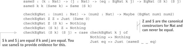
Unlike ==, checkEqNat expresses the relationship between its inputs and its output precisely in its type. Using this, we can make another attempt to implement exact-Length.
8.1.5. Implementing exactLength, second attempt
Earlier, we reached the following point in implementing exactLength, before establishing that a Boolean comparison wasn’t sufficient:
exactLength : (len : Nat) -> (input : Vect m a) -> Maybe (Vect len a) exactLength {m} len input = case m == len of False => ?exactLength_rhs_1 True => ?exactLength_rhs_2 Instead of using the Boolean comparison operator == to compare m and len, you can try using checkEqNat m len. This will return a value of type Maybe (EqNat m len), so if m and len are equal, you’ll have some additional information in the type that states the meaning of the result of the comparison precisely. In this second attempt, you can implement the function as follows:
- Define— As before, begin with a type and a skeleton definition, bringing m into scope on the left side:
exactLength : (len : Nat) -> (input : Vect m a) -> Maybe (Vect len a) exactLength {m} len input = ?exactLength_rhs - Define— Instead of defining the function by case splitting on the result of m == len, case-split on the result of checkEqNat:
exactLength : (len : Nat) -> (input : Vect m a) -> Maybe (Vect len a) exactLength {m} len input = case checkEqNat m len of Nothing => ?exactLength_rhs_1 Just eq_nat => ?exactLength_rhs_2 - Refine— If checkEqNat returns Nothing, the inputs were different, so the input vector is the wrong length:
exactLength : (len : Nat) -> (input : Vect m a) -> Maybe (Vect len a) exactLength {m} len input = case checkEqNat m len of Nothing => Nothing Just eq_nat => Just ?exactLength_rhs_2 - Type— If checkEqNat returns Just eq_nat, the lengths are equal, and eq_nat provides evidence that they’re equal. For ?exactLength_rhs_2, you have this:
m : Nat len : Nat eq_nat : EqNat m len a : Type input : Vect m a -------------------------------------- exactLength_rhs_2 : Maybe (Vect len a)
- Define— As before, you still need to provide a result of type Maybe (Vect len a), and all you have available is input of type Vect m a. But you also have eq_nat, which provides evidence that m and len are equal. If you case-split on eq_nat, you’ll get the following:
exactLength : (len : Nat) -> (input : Vect m a) -> Maybe (Vect len a) exactLength {m} len input = case checkEqNat m len of Nothing => Nothing Just (Same len) => ?exactLength_rhs_1Then, when inspecting the type of the new hole, ?exactLength_rhs_1, you’ll see this:m : Nat a : Type input : Vect len a -------------------------------------- exactLength_rhs_1 : Maybe (Vect len a)
Because eq_nat can only take the form Same len, and the type of Same len forces m to be identical to len, Idris has refined the required type to be Maybe (Vect len a). - Refine— From here, it’s easy to complete the definition:
exactLength : (len : Nat) -> (input : Vect m a) -> Maybe (Vect len a) exactLength {m} len input = case checkEqNat m len of Nothing => Nothing Just (Same len) => Just input
8.1.6. Equality in general: the = type
Rather than defining a specific equality type and function for every possible type you’ll need to compare, such as Nat with EqNat and checkEqNat here, Idris provides a generic equality type. This is built into Idris’s syntax, so you can’t define this yourself (because = is a reserved symbol), but conceptually it would be defined as follows.
Listing 8.4. Conceptual definition of a generic equality type
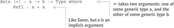
The name Refl is short for reflexive, a mathematical term that (informally) means that a value is equal to itself. As with EqNat, you can try some examples at the REPL:
Idris> the ("Hello" = "Hello") Refl Refl : "Hello" = "Hello" Idris> the (True = True) Refl Refl : True = True If you give more-complex expressions as part of the type, Idris will evaluate them. For example, if you give the expression 2 + 2 as part of a type, 2 + 2 = 4, Idris will evaluate it:
Idris> the (2 + 2 = 4) Refl Refl : 4 = 4
As before, if you try to use Refl to build an instance of an equality type using two unequal values, you’ll get an error:
Idris> the (True = False) Refl (input):1:5:When checking argument value to function Prelude.Basics.the: Type mismatch between x = x (Type of Refl) and True = False (Expected type) Specifically: Type mismatch between True and False
Using the built-in equality type, rather than EqNat, you can define checkEqNat as follows.
Listing 8.5. Checking equality between Nats using the generic equality type (CheckEqMaybe.idr)
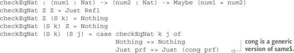
cong : {func : a -> b} -> x = y -> func x = func y In other words, given some (implicit) function, func, if you have two values that are equal, then applying func to those values gives an equal result. This does the same job as sameS, using the generic equality type.
Exercises
- Implement the following function, which states that if you add the same value onto the front of equal lists, the resulting lists are also equal:
same_cons : {xs : List a} -> {ys : List a} -> xs = ys -> x :: xs = x :: ysBecause this function represents an equality proof, it’s sufficient to know that your definition type-checks and is total:*ex_8_1> :total same_cons Main.same_cons is Total
- Implement the following function, which states that if two values, x and y, are equal, and two lists, xs and ys, are equal, then the two lists x :: xs and y :: ys must also be equal:
same_lists : {xs : List a} -> {ys : List a} -> x = y -> xs = ys -> x :: xs = y :: ysAgain, it’s sufficient to know that your definition type-checks. - Define a type, ThreeEq, that expresses that three values must be equal. Hint: ThreeEq should have the type a -> b -> c -> Type.
- Implement the following function, which uses ThreeEq:
allSameS : (x, y, z : Nat) -> ThreeEq x y z -> ThreeEq (S x) (S y) (S z)
What does this type mean?
8.2. Equality in practice: types and reasoning
Equality proofs, and functions that manipulate them, can be useful when defining functions with dependent types. You saw a small example of this when implementing checkEqNat, where you wrote a sameS function to show that adding one to equal numbers results in equal numbers.Reasoning about equality often becomes necessary when writing functions on types that are indexed by numbers. For example, when manipulating vectors, you might need to prove the equivalence between two expressions with natural numbers that appear in the types of the vectors. To see how this can happen and how to deal with it, we’ll look at how to implement a function that reverses a Vect.
8.2.1. Reversing a vector
If you import Data.Vect, you’ll get access to a function that reverses a vector, with the following type:
reverse : Vect n elem -> Vect n elem
The type states that reversing a vector preserves the length of the input vector. You’d expect it to be fairly straightforward to implement this function using the following rules:
- If the input vector is empty, return an empty vector.
- If the input vector isn’t empty and has a head x and a tail xs, reverse xs and append x.
Let’s see what happens if we try to implement our own version, myReverse, in the file ReverseVec.idr:
- Type, define— Begin with a type and a skeleton definition, and case-split on the input:
myReverse : Vect n elem -> Vect n elem myReverse [] = ?myReverse_rhs_1 myReverse (x :: xs) = ?myReverse_rhs_2
- Refine— For ?myReverse_rhs_1, return an empty vector:
myReverse : Vect n elem -> Vect n elem myReverse [] = [] myReverse (x :: xs) = ?myReverse_rhs_2
- Refine failure—For ?myReverse_rhs_2, you’d like to be able to reverse xs and append x, as follows, but unfortunately this fails:
The error message tells you that Idris has found a mismatch between the type of the value you’ve given, Vect (k + 1), and the expected type, Vect (S k):
ReverseVec.idr:6:12: When checking right hand side of myReverse with expected type Vect (S k) elem Type mismatch between Vect (k + 1) elem (Type of myReverse xs ++ [x]) and Vect (S k) elem (Expected type)
This seems surprising, because our knowledge of the behavior of addition suggests that S k and k + 1 will always evaluate to the same result, whatever the value of k.
We’ll postpone the completion of this definition and take a closer look at how type checking works in Idris in order to understand what has gone wrong and how we might correct it.
8.2.2. Type checking and evaluation
When Idris type-checks an expression, it will look at the expected type of the expression, and check that the type of the given expression matches it, after evaluating both. The following code fragment will type-check:
test1 : Vect 4 Int test1 = [1, 2, 3, 4] test2: Vect (2 + 2) Int test2 = test1
Even though test1 and test2 have different expressions in their types, these expressions evaluate to the same result, so you can define test2 to return test1.
You can see at the REPL how the Idris type checker evaluates types containing type variables by using an anonymous function (explained in chapter 2) to introduce variables with unknown values. Consider this example:
*ReverseVec> \k, elem => Vect (1 + k) elem \k => \elem => Vect (S k) elem : Nat -> Type -> Type
Here, Idris has evaluated 1 + k in the type to S k. But if you try swapping the arguments to +, you’ll get a different result:
*ReverseVec> \k, elem => Vect (k + 1) elem \k => \elem => Vect (plus k 1) elem : Nat -> Type -> Type
Here, Idris has evaluated k + 1 to plus k 1, where plus is the Prelude function that implements addition on Nat. To see the reason for the difference, you need to look at the definition of plus. You can do this using the REPL command :printdef, which prints the pattern-matching definition of the function given as its argument:
*ReverseVec> :printdef plus plus : Nat -> Nat -> Nat plus 0 right = right plus (S left) right = S (plus left right)Because plus is defined by pattern-matching on its first argument, Idris can’t evaluate plus k 1 any further. To do so, it would need to know what form k takes, but at the moment, neither of the clauses for plus matches.
Returning to our problem with defining myReverse, let’s take a look at the current state:

If you rewrite the definition using let to build each component of the result, and leave a hole for the return value, you can see in more detail what problem you have to solve:
myReverse : Vect n elem -> Vect n elem myReverse [] = [] myReverse (x :: xs) = let rev_xs = myReverse xs result = rev_xs ++ [x] in ?myReverse_rhs_2
Checking the type of ?myReverse_rhs_2 shows the type of each component and the required type of the result:
elem : Type x : elem k : Nat xs : Vect k elem rev_xs : Vect k elem result : Vect (plus k 1) elem -------------------------------------- myReverse_rhs_2 : Vect (S k) elem
For the intended result, you have an expression with type Vect (k + 1) elem, but you need an expression with type Vect (S k) elem.
You know, from trying the evaluation at the REPL previously, that Vect (1 + k) elem would evaluate to the type you need, so you need to be able to explain to Idris that 1 + k is equal to k + 1; or, when evaluated, that S k is equal to plus k 1. The Idris library provides a function that can help you:
plusCommutative : (left : Nat) -> (right : Nat) -> left + right = right + left
If you check the type of plusCommutative at the REPL with values 1 and k for left and right, respectively, you’ll see exactly the equality you need:
*ReverseVec> :t \k => plusCommutative 1 k \k => plusCommutative 1 k : (k : Nat) -> S k = plus k 1
You can think of this expression’s type as a “rewrite rule” that allows you to replace one value with another. If you can find a way to apply this rule to rewrite the expected type to Vect (plus k 1) a, you’ll be able to complete the definition.
8.2.3. The rewrite construct: rewriting a type using equality
We’ll resume our definition of myReverse at the following point, using let to name the result we’d like to return:myReverse : Vect n elem -> Vect n elem myReverse [] = [] myReverse (x :: xs) = let result = myReverse xs ++ [x] in ?myReverse_rhs_2
At this stage, these are the types:
elem : Type x : elem k : Nat xs : Vect k elem result : Vect (plus k 1) elem -------------------------------------- myReverse_rhs_2 : Vect (S k) elem
In order to complete the definition, you can use the information given by plus-Commutative 1 k to rewrite the type of ?myReverse_rhs_2. You’ll want to replace any S k in the type of ?myReverse_rhs_2 with plus k 1, so that you can return result. Idris provides a syntax for using equality proofs to rewrite types, illustrated in figure 8.1.
Figure 8.1. Rewriting a type using an equality proof
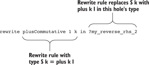
You can therefore implement myReverse using the rewrite construct to update the type of ?myReverse_rhs_2, taking the following steps:
- Define— Before rewriting the type using plusCommutative 1 k, you’ll need to bring k into scope, and k arises from pattern matching on the length of the input vector:
myReverse : Vect n elem -> Vect n elem myReverse [] = [] myReverse {n = S k} (x :: xs) = let result = myReverse xs ++ [x] in ?myReverse_rhs_2 - Refine, type— Now, you can apply the rewriting rule:
myReverse : Vect n elem -> Vect n elem myReverse [] = [] myReverse {n = S k} (x :: xs) = let result = myReverse xs ++ [x] in rewrite plusCommutative 1 k in ?myReverse_rhs_2If you look at the resulting type for ?myReverse_rhs_2, you can see the effect the rewrite has had:elem : Type k : Nat x : elem xs : Vect k elem result : Vect (plus k 1) elem _rewrite_rule : plus k 1 = S k -------------------------------------- myReverse_rhs_2 : Vect (plus k 1) elem
- Refine— Finally, you can complete the definition using expression search:
myReverse : Vect n elem -> Vect n elem myReverse [] = [] myReverse {n = S k} (x :: xs) = let result = myReverse xs ++ [x] in rewrite plusCommutative 1 k in result
Using rewrite, you’ve replaced an expression in the type (S k) with an equivalent expression (plus k 1), which allows you to use result. But although this has allowed you to write the function, this definition still leaves something to be desired: the part of the definition that computes the result (myReverse xs ++ [x]) has become rather lost in the details of the proof. You can improve this by delegating the details of the proof, using a hole.
8.2.4. Delegating proofs and rewriting to holes
Instead of applying the rewrite inside the definition of myReverse, you can use a hole along with interactive editing to generate a helper function that contains the details of the proof. Let’s start again, with our initial (failing) definition of myReverse:
myReverse : Vect n elem -> Vect n elem myReverse [] = [] myReverse (x :: xs) = myReverse xs ++ [x]
You can correct this definition using the following steps:
- Refine, type— Add a hole to the right side, which takes the initial attempt as an argument:
myReverse : Vect n elem -> Vect n elem myReverse [] = [] myReverse (x :: xs) = ?reverseProof (myReverse xs ++ [x])
If you check the type of ?reverseProof, you’ll see exactly how you need to rewrite the type for this definition to be accepted:elem : Type x : elem k : Nat xs : Vect k elem -------------------------------------- reverseProof : Vect (plus k 1) elem -> Vect (S k) elem
- Type— Using Ctrl-Alt-L in Atom, lift ?reverseProof to a top-level function:
reverseProof : (x : elem) -> (xs : Vect k elem) -> Vect (k + 1) elem -> Vect (S k) elem myReverse : Vect n elem -> Vect n elem myReverse [] = [] myReverse (x :: xs) = reverseProof x xs (myReverse xs ++ [x])
- Define— Define reverseProof as follows, using the same application of rewrite as in your previous definition of myReverse:
reverseProof : (x : elem) -> (xs : Vect k elem) -> Vect (k + 1) elem -> Vect (S k) elem reverseProof {k} x xs result = rewrite plusCommutative 1 k in result - Refine— Finally, because you don’t use x or xs in reverseProof, and because reverseProof will only be used by myReverse, you can tidy up the definition as follows:
myReverse : Vect n elem -> Vect n elem myReverse [] = [] myReverse (x :: xs) = reverseProof (myReverse xs ++ [x]) where reverseProof : Vect (k + 1) elem -> Vect (S k) elem reverseProof {k} result = rewrite plusCommutative 1 k in result
By introducing the hole ?reverseProof, you’ve been able to keep the relevant computation part of myReverse separate from the details of the proof.
8.2.5. Appending vectors, revisited
You can often avoid the need for rewriting in types by taking care in how you write function types. For example, in chapter 4, you saw how to define a function that appends vectors with the following type:
append : Vect n elem -> Vect m elem -> Vect (n + m) elem
The order of arguments to the + operator in the return type turns out to be important because of the definition of +. If you begin to implement this (in the file AppendVec.idr) by creating a skeleton definition and then case splitting on the first argument, you’ll reach the following state:
append : Vect n elem -> Vect m elem -> Vect (n + m) elem append [] ys = ?append_rhs_1 append (x :: xs) ys = ?append_rhs_2
Then, if you check the type of ?append_rhs_1, you’ll see the following:
elem : Type m : Nat ys : Vect m elem -------------------------------------- append_rhs_1 : Vect m elem
In this case, the first argument, [], has type Vect 0 elem, and the second argument, ys, has type Vect m elem. According to the return type of append, ?append_rhs_1 should have type Vect (0 + m) elem, which reduces to Vect m elem by the definition of +.
Take a look at what happens if you swap the arguments n and m, as follows:
append : Vect n elem -> Vect m elem -> Vect (m + n) elem append [] ys = ?append_rhs_1 append (x :: xs) ys = ?append_rhs_2
You now see a different type for ?append_rhs_1:
elem : Type m : Nat ys : Vect m elem -------------------------------------- append_rhs_1 : Vect (plus m 0) elem
As in the definition of myReverse, Idris can’t reduce plus m 0 any further, because plus is defined by pattern-matching on its first argument, and the form of m is unknown. Because of this, you can’t simply return ys for this case, and you’ll need to rewrite the type of append_rhs_1. You’ll have a similar problem for append_rhs_2; the following listing shows the definition of append, with holes in place of the necessary rewrites.
Listing 8.6. Implementing append on vectors with the arguments to + swapped in the return type (AppendVec.idr)
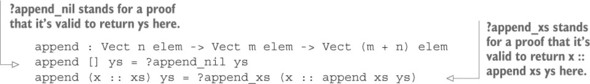
The next listing shows a completed definition of append, with definitions of append_nil and append_xs that rewrite the types for each case.
Listing 8.7. Completing append on vectors by adding rewriting proofs for append_nil and append_xs (AppendVec.idr)
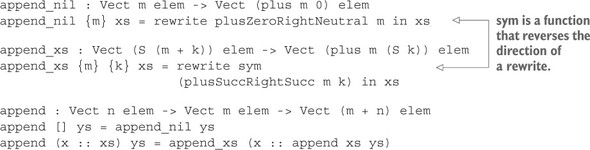
plusZeroRightNeutral : (left : Nat) -> left + 0 = left plusSuccRightSucc : (left : Nat) -> (right : Nat) -> S (left + right) = left + S right
The third, sym, allows you to apply a rewrite rule in reverse:
sym : left = right -> right = left
Essentially, plusZeroRightNeutral and plusSuccRightSucc together explain that the behavior of plus is identical if the arguments are given in the opposite order.
Exercises
- Using plusZeroRightNeutral and plusSuccRightSucc, write your own version of plusCommutes:
myPlusCommutes : (n : Nat) -> (m : Nat) -> n + m = m + n
Hint: Write this by case splitting on n. In the case of S k, you can rewrite with a recursive call to myPlusCommutes k m, and rewrites can be nested. - The implementation of myReverse you wrote earlier is inefficient because it needs to traverse the entire vector to append a single element on every iteration. You can write a better definition as follows, using a helper function, reverse', that takes an accumulating argument to build the reversed list:
myReverse : Vect n a -> Vect n a myReverse xs = reverse' [] xs where reverse' : Vect n a -> Vect m a -> Vect (n+m) a reverse' acc [] = ?reverseProof_nil acc reverse' acc (x :: xs) = ?reverseProof_xs (reverse' (x::acc) xs)
Complete this definition by implementing the holes ?reverseProof_nil and ?reverseProof_xs. You can test your answer at the REPL as follows:*ex_8_2> myReverse [1,2,3,4] [4, 3, 2, 1] : Vect 4 Integer
8.3. The empty type and decidability
You can use the equality type, =, to write functions with types that state that two values are guaranteed to be equal, and then use this guarantee elsewhere in the program. This works because the only way to construct a value with an equality type is to use Refl, and Refl will only construct a value with a type of the form x = x:
Idris> :t Refl Refl : x = x Idris> Refl {x = 94} Refl : 94 = 94 But what if you want to say the opposite, that two values are guaranteed not to be equal? When you construct a value in a type, you’re effectively giving evidence that an element of that type exists. To show that two values x and y are not equal, you need to be able to give evidence that an element of the type x = y can’t exist. In this section, you’ll see how to use the empty type, Void, to express that something is impossible. If a function returns a value of type Void, that can only mean that it’s impossible to construct values of its inputs (or, logically, that the types of its inputs express a contradiction.) We’ll use Void to express guarantees in types that values can’t be equal, and then use it to write a more precise type for checkEqNat, which guarantees that
- If its inputs are equal, it will produce a proof that they are equal
- If its inputs are not equal, it will produce a proof that they are not equal
First, let’s take a look at how Void is defined and used in the simplest case.
8.3.1. Void: a type with no values
In order to express that something can’t happen, the Prelude provides a type with no values, Void. The complete definition of Void is as follows:
data Void : Type where
You can’t write values of type Void directly, because there aren’t any! As a result, if you have a function that returns something of type Void, it must be because one of its arguments is also impossible to construct.
Just as you can use = to write functions that express facts about how functions do behave, you can use Void to express facts about how functions don’t behave. For example, you can show that 2 + 2 doesn’t equal 5.
Let’s write a function in a file named Void.idr:
- Type— Begin by writing the appropriate type:
twoPlusTwoNotFive : 2 + 2 = 5 -> Void
You can read this “if 2 + 2 = 5, then return an element of the empty type.” - Define— Adding a skeleton definition gives you this:
twoPlusTwoNotFive : 2 + 2 = 5 -> Void twoPlusTwoNotFive prf = ?twoPlusTwoNotFive_rhs
If you look at the type of prf, you’ll see that it’s a proof that 4 = 5:prf : 4 = 5 -------------------------------------- twoPlusTwoNotFive_rhs : Void
- Define— You can try to define the function by a case split on prf. Idris produces this:
twoPlusTwoNotFive : 2 + 2 = 5 -> Void twoPlusTwoNotFive Refl impossible
This definition is now complete. Idris has produced one case, and noticed that the only possible input, Refl, can never be valid. Recall from chapter 4 that the impossible keyword means that the pattern clause must not type-check.
It’s important to check that a function that returns Void is a total function, if you really want to believe that it takes an impossible input:
*Void> :total twoPlusTwoNotFive Main.twoPlusTwoNotFive is Total
Otherwise, you could write a function that claims to return Void by looping forever:
loop : Void loop = loop
This function isn’t total, so you can’t believe that it really does produce an element of Void. Idris reports the following:
*Void> :total loop Main.loop is possibly not total due to recursive path: Main.loop
Similarly, you can write a function that shows that a number can never be equal to its successor:
valueNotSuc : (x : Nat) -> x = S x -> Void valueNotSuc _ Refl impossible
If you were able to provide a value of the empty type, you’d be able to produce a value of any type. In other words, if you have a proof that an impossible value has happened, you can do anything. The Prelude provides a function, void, that expresses this:
void : Void -> a
It may seem strange, and of little practical use, to be writing functions merely to show that something can’t happen. But if you know that something can’t happen, you can use this knowledge to express limitations about what can happen. In other words, you can express more precisely what a function is intended to do.
8.3.2. Decidability: checking properties with precision
Previously, when you wrote checkEqNat, you used Maybe for the result:
checkEqNat : (num1 : Nat) -> (num2 : Nat) -> Maybe (num1 = num2)
So, if checkEqNat returns a value of the form Just p, you can be certain that num1 and num2 are equal, and that p represents a proof that they’re equal. But you can’t say the opposite: that if checkEqNat returns Nothing, then num1 and num2 are guaranteed not to be equal.
The following definition would, for example, be perfectly valid, though not very useful:
checkEqNat : (num1 : Nat) -> (num2 : Nat) -> Maybe (num1 = num2) checkEqNat num1 num2 = Nothing
Instead, to make this type more precise, you’d need a way of stating that for any pair of numbers, num1 and num2, you’ll always be able to produce either a proof that they’re equal (of type num1 = num2) or a proof that they’re not equal (of type num1 = num2 -> Void). That is, you’d like to state that checking whether num1 = num2 is a decidable property.
Decidability
A property of some values is decidable if you can always say whether the property holds or not for specific values. For example, checking equality on Nat is decidable, because for any two natural numbers you can always decide whether they are equal or not.
Listing 8.8 shows the Dec generic type, which is defined in the Prelude. Like Maybe, Dec has a constructor (Yes) that carries a value. Unlike Maybe, it also has a constructor (No) that carries a proof that no value of its argument type can exist.
Listing 8.8. Dec: precisely stating that a property is decidable
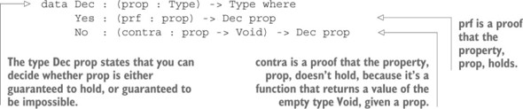
For example, you can construct a proof that 2 + 2 = 4, so you’d use Yes:
*Void> the (Dec (2 + 2 = 4)) (Yes Refl) Yes Refl : Dec (4 = 4)
But it’s impossible to construct a proof that 2 + 2 = 5, so you’d use No and provide your evidence, twoPlusTwoNotFive, that it’s impossible:
*Void> the (Dec (2 + 2 = 5)) (No twoPlusTwoNotFive) No twoPlusTwoNotFive : Dec (4 = 5)
Let’s rewrite checkEqNat using Dec instead of Maybe for the result type. In doing so, we’ll have two guarantees verified by the Idris type checker:
- If the inputs num1 and num2 are equal, checkEqNat is guaranteed to produce a result of the form Yes prf, where prf has type num1 = num2.
- If the inputs num1 and num2 are not equal, checkEqNat is guaranteed to produce a result of the form No contra, where contra has type num1 = num2 -> Void.
These are guarantees because the type of checkEqNat gives a direct link between the inputs and the output type:
checkEqNat : (num1 : Nat) -> (num2 : Nat) -> Dec (num1 = num2)
You can write this function interactively, in a new file called CheckEqDec.idr:
- Define, refine— You can mostly follow the same steps as earlier, when you defined checkEqNat using Maybe. But instead of Just, use Yes, and instead of Nothing, use No. No requires proofs that the inputs are unequal, so you can leave holes for these for the moment:
checkEqNat : (num1 : Nat) -> (num2 : Nat) -> Dec (num1 = num2) checkEqNat Z Z = Yes Refl checkEqNat Z (S k) = No ?zeroNotSuc checkEqNat (S k) Z = No ?sucNotZero checkEqNat (S k) (S j) = case checkEqNat k j of Yes prf => Yes (cong prf) No contra => No ?noRec
You can test this at the REPL, even without the proofs, though you may see holes in the results:*CheckEqDec> checkEqNat 3 3 Yes Refl : Dec (3 = 3) *CheckEqDec> checkEqNat 3 4 No ?noRec : Dec (3 = 4) *CheckEqDec> checkEqNat 3 0 No ?sucNotZero : Dec (3 = 0)
- Type— If you look at the types of the holes, you’ll see what you need to prove to complete the definition, as in this example:
k : Nat -------------------------------------- zeroNotSuc : (0 = S k) -> Void
- Define, refine— You can lift ?zeroNotSuc and ?sucNotZero to top-level definitions with Ctrl-Alt-L and implement them using case splitting and impossible, as with twoPlusTwoNotFive in the previous section, because it’s never possible for zero to be equal to a nonzero number:
zeroNotSuc : (0 = S k) -> Void zeroNotSuc Refl impossible sucNotZero : (S k = 0) -> Void sucNotZero Refl impossible
- Type, define— For ?noRec, you can take a look at the type to see what you need to show:
k : Nat j : Nat contra : (k = j) -> Void -------------------------------------- noRec : (S k = S j) -> Void
The type of contra tells you that k is guaranteed not to be equal to j. Given that, you have to show that S k can’t equal S j. Again, you can lift this to a top-level definition with Ctrl-Alt-L:noRec : (contra : (k = j) -> Void) -> (S k = S j) -> Void noRec contra prf = ?noRec_rhs
- Define— The type of noRec says that if you have a proof that k = j is impossible, and a proof that S k = S j, you can produce an element of the empty type. Logically, the two inputs contradict each other. You can write this function by case splitting on prf:
noRec : (contra : (k = j) -> Void) -> (S k = S j) -> Void noRec contra Refl = ?noRec_rhs_1
- Type— The only possible value prf can take is Refl, and the only way it can take the value Refl is if S k and S j are equal, and therefore k and j are equal. Recognizing this, Idris refines the type of contra, as you can see by inspecting the type of noRec_rhs_1:
j : Nat contra : (j = j) -> Void -------------------------------------- noRec_rhs_1 : Void
- Refine— To complete the definition, you can use contra to produce an element of the empty type; an expression search will find this:
noRec : (contra : (k = j) -> Void) -> (S k = S j) -> Void noRec contra Refl = contra Refl
The following listing shows the complete definition of checkEqNat, including the helper functions zeroNotSuc, sucNotZero, and noRec.
Listing 8.9. Checking whether Nats are equal, with a precise type (CheckEqDec.idr)
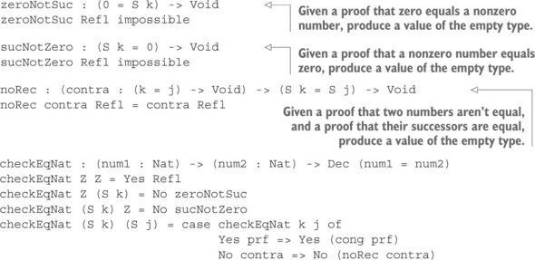
Proving inputs are impossible with Void
When you run checkEqNat, you aren’t really going to produce a value of the empty type using zeroNotSuc, sucNotZero, or noRec. Essentially, a function that produces a value of type Void can be seen as a proof that its arguments can’t all be provided at the same time. In the case of noRec, the type of the functions says that if you can provide both a proof that k doesn’t equal j and a proof that S k = S j, then there’s a contradiction, and you can therefore have a value of type Void.By using Dec, you’ve been able to write explicitly in the type what checkEqNat is supposed to do: return either a proof that the inputs are equal or a proof that they’re not. The real benefit of this comes not in checkEqNat itself, however, but in the functions that use it, because they not only have the result of the equality test, but also a proof that the equality test has worked correctly.
Being able to guarantee that two values are equal (or different) is commonly useful in type-driven development, because showing relationships between larger structures depends on showing relationships between the individual components. Because of this, the Idris Prelude provides an interface, DecEq, with a generic function, decEq, for deciding equality.
8.3.3. DecEq: an interface for decidable equality
Rather than providing specific functions like checkEqNat for each type, the Idris Prelude provides an interface, DecEq. The next listing shows how DecEq is defined. There are implementations for all of the types defined in the Prelude.
Listing 8.10. The DecEq interface (defined in the Prelude)

Instead of defining and using a special-purpose function, checkEqNat, to define exact-Length, you could use decEq. The following listing shows how to do this, and it’s the definition of exactLength used in Data.Vect.
Listing 8.11. Implementing exactLength using decEq (ExactLengthDec.idr)
exactLength : (len : Nat) -> (input : Vect m a) -> Maybe (Vect len a) exactLength {m} len input = case decEq m len of Yes Refl => Just input No contra => Nothing Using decEq rather than the Boolean equality operator, ==, gives you a strong guarantee about how the equality test works. You can be sure that if decEq returns a value of the form Yes prf, then the inputs really are structurally equal. In the next chapter, you’ll see how to describe relationships between larger data structures (such as showing that a value is an element of a list) and how to use decEq to build proofs of these relationships.
Exercises
- Implement the following functions:
headUnequal : DecEq a => {xs : Vect n a} -> {ys : Vect n a} -> (contra : (x = y) -> Void) -> ((x :: xs) = (y :: ys)) -> Void tailUnequal : DecEq a => {xs : Vect n a} -> {ys : Vect n a} -> (contra : (xs = ys) -> Void) -> ((x :: xs) = (y :: ys)) -> VoidThe first states that if the first elements of two vectors are unequal, then the vectors must be unequal. The second states that if there are differences in the tails of two vectors, then the vectors must be unequal. If you have a correct solution, both headUnequal and tailUnequal should type-check and be total:*ex_8_3> :total headUnequal Main.headUnequal is Total *ex_8_3> :total tailUnequal Main.tailUnequal is Total
- Implement DecEq for Vect. Begin with the following implementation header:
DecEq a => DecEq (Vect n a) where
Hint: You’ll find headUnequal and tailUnequal useful here. Remember to check the types of the holes as you write the definition. You should also use your own definition of Vect rather than importing Data.Vect, because the library provides a DecEq implementation. You can test your answer at the REPL as follows:*ex_8_3> decEq (the (Vect _ _) [1,2,3]) [1,2,3] Yes Refl : Dec ([1, 2, 3] = [1, 2, 3])
8.4. Summary
- You can write a type to express a proof that two values must be equal.
- You can write functions that take equality types as inputs to prove additional properties of data.
- Using Maybe, you can test for equality of values at runtime.
- The generic = type allows you to describe equality between values of any type.
- Proof requirements arise naturally when programming with dependent types, such as to show that lengths are preserved when reversing a vector.
- The rewrite construct allows you to update a type using an equality proof.
- Using holes and interactive editing, you can delegate the details of rewriting types to a separate function.
- Void is a type with no values, used to show that inputs to a function can’t all occur at once.
- A property is decidable if you can always say whether the property holds for some specific values.
- Using Dec, you can compute at runtime whether a property is guaranteed to hold or guaranteed not to hold.
Chapter 9. Predicates: expressing assumptions and contracts in types
This chapter covers
- Describing and checking membership of a vector using a predicate
- Using predicates to describe contracts for function inputs and outputs
- Reasoning about system state in types
Dependent types like EqNat and =, which you saw in the previous chapter, are used entirely for describing relationships between data. These types are often referred to as predicates, which are data types that exist entirely to describe a property of some data. If you can construct a value for a predicate, then you know the property described by that predicate must be true.
In this chapter, you’ll see how to express more-complex relationships between data using predicates. By expressing relationships between data in types, you can be explicit about the assumptions you’re making about the inputs to a function, and have those assumptions checked by the type checker when those functions are
called. You can even think of these assumptions as expressing compile time contracts that other arguments must satisfy before anything can call the function.In practice, you’ll often write functions that make assumptions about the form of some other data, having (hopefully!) checked those assumptions beforehand. Here are a few examples:
- A function that reads from a file assumes that the file handle describes an open file.
- A function that processes data it has received from a network assumes that the data follows the appropriate protocol.
- A function that retrieves user data (say, for a customer on a website) assumes that the user has successfully authenticated.
You need to ensure that you check any necessary assumptions before you call these functions, particularly when security or user privacy is at stake. In Idris, you can make this kind of assumption explicit in a type, and have the type checker ensure that you’ve properly checked the assumption in advance. An advantage of expressing assumptions in types is that they are guaranteed to hold, even as a system evolves over time.
In this chapter, we’ll take an in-depth look at a specific small example: removing a value from a vector if that value is contained within the vector. We’ll look at how to express in a type that a vector contains a specific element, how to test this property at runtime, and how to use such properties in practice to write a larger program with some aspects of its behavior expressed in its types.
9.1. Membership tests: the Elem predicate
Using =, Void, and Dec, you can describe properties that your programs satisfy in their types, making the types precise as a result. Typically, you’ll use =, Void, and Dec as building blocks for describing and checking relationships between pieces of data. Describing relationships in types allows you to state assumptions that functions make and, more importantly, it allows Idris to check whether those assumptions are satisfied or violated.
For example, you might want to
- Remove an element from a vector only under the assumption that the element is present in the vector
- Search for a value in a list only under the assumption that the list is ordered
- Run a database query only under the assumption that the inputs have been validated
- Send a message to a machine on the network only under the assumption that you have an open connection
In this section, we’ll examine the first of these in more detail. We’ll begin by trying to write a function that removes an element from a vector, and then we’ll see how we can refine the type to state and check any necessary assumptions that make the type more precise. Finally, we’ll use the function in a simple interactive program.
9.1.1. Removing an element from a Vect
If you have a Vect containing a number of elements, you’d expect the following of a removeElem function that removes a specific element from that vector:- The input vector should have at least one element.
- The output vector’s length should be one less than the input vector’s length.
Because Vect is parameterized by the element type contained in the vector and is indexed by the length of the vector, you can (indeed, you must) express these length properties in the type of removeElem. Your first attempt might look like this:
removeElem : (value : a) -> (xs : Vect (S n) a) -> Vect n a
Let’s see what happens if you try to write this function:
- Define— If you add a skeleton definition and case-split on xs, Idris will give you only one pattern, because xs can’t be an empty vector:
removeElem : (value : a) -> (xs : Vect (S n) a) -> Vect n a removeElem value (x :: xs) = ?removeElem_rhs_1
- Refine— If the value you’re looking for is equal to x, you can remove it from the list, returning xs. You’ll need to refine the type before you can compare value and x; you can use decidable equality so that you can be certain that the equality test is accurate. This is the refined type:
removeElem : DecEq a => (value : a) -> (xs : Vect (S n) a) -> Vect n a
- Refine— You can now use decEq to compare value and x, and discard x if they’re equal:
removeElem : DecEq a => (value : a) -> (xs : Vect (S n) a) -> Vect n a removeElem value (x :: xs) = case decEq value x of Yes prf => xs No contra => ?removeElem_rhs_3
- Refine failure—For ?removeElem_rhs_3, you might hope to be able to remove value from xs recursively, but if you try this, you’ll get an error:
removeElem : DecEq a => (value : a) -> (xs : Vect (S n) a) -> Vect n a removeElem value (x :: xs) = case decEq value x of Yes prf => xs No contra => x :: removeElem value xs
Idris reports the following:When checking right hand side of Main.case block in removeElem at removeelem.idr:4:35 with expected type Vect n a When checking argument xs to Main.removeElem: Type mismatch between Vect n a (Type of xs) and Vect (S k) a (Expected type)
The problem is that removeElem requires a vector that’s guaranteed to be non-empty, but xs may be empty! You can see this from its type, Vect n a: the n could stand for any natural number, including zero. This problem arises because there’s no guarantee that value will appear in the vector, so it’s possible to reach the end of the vector without encountering it. If this happens, there’s no value to remove, so you can’t satisfy the type. You’ll need to refine the type further in order to be able to write this function. You can try one of the following:- Rewrite the type so that removeElem returns Maybe (Vect n a), returning Nothing if the value doesn’t appear in the input.
- Rewrite the type so that removeElem returns a dependent pair, (newLength ** Vect newLength a).
- Express a precondition on removeElem that the value is guaranteed to be in the vector.
You’ve already seen how to express possible failure with Maybe (in chapter 4), and how to express an unknown length using dependent pairs (in chapter 5). The third option, however, would express the purpose of removeElem precisely. To achieve this, you’ll need to write a type that describes the relationship between a value and a vector that contains that value.
If you can describe in a type that a vector contains a specific element, you’ll be able to use that type to express a contract on removeElem expressing that you can only use it if you know the element is in the vector. In the rest of this section, you’ll implement this type, Elem, use it to make the type of removeElem more precise, and learn more about how to use Elem in practice.
9.1.2. The Elem type: guaranteeing a value is in a vector
In the previous chapter, you saw how to express that two values are guaranteed to be equal by using either a specific EqNat type or the generic = type. The existence of a value in one of these types is, essentially, a proof that two values are equal. You can do something similar to guarantee that a value is in a vector.
Our goal is to define a type, Elem, with the following type constructor:
Elem : (value : a) -> (xs : Vect k a) -> Type
If we have a value, and a vector, xs, that contains that value, we should be able to construct an element of the type Elem value xs. For example, we should be able to construct the following:
oneInVector : Elem 1 [1,2,3] maryInVector : Elem "Mary" ["Peter", "Paul", "Mary"]
We should also be able to construct functions of the following types, which show that a specific value is not contained in a vector:
fourNotInVector : Elem 4 [1,2,3] -> Void peteNotInVector : Elem "Pete" ["John", "Paul", "George", "Ringo"] -> VoidThe following listing shows how the Elem dependent type is defined in Data.Vect.
Listing 9.1. The Elem dependent type, expressing that a value is guaranteed to be contained in a vector (defined in Data.Vect)
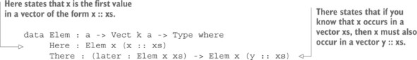
The value Here can be read as a proof that a value is the first value in a vector, as in this example:
oneInVector : Elem 1 [1,2,3] oneInVector = Here
The constructor There, given an argument that shows a value x is in the vector xs, can be read as a proof that x must also be in the vector y :: xs for any value y.
To illustrate this, let’s try to write maryInVector:
maryInVector : Elem "Mary" ["Peter", "Paul", "Mary"]
- Define— Create a skeleton definition with a hole for the right side:
maryInVector : Elem "Mary" ["Peter", "Paul", "Mary"] maryInVector = ?maryInVector_rhs
- Refine, type—You can’t use Here, because "Mary" isn’t the first element of the vector, so try using There and leaving a hole for its argument:
maryInVector : Elem "Mary" ["Peter", "Paul", "Mary"] maryInVector = There ?maryInVector_rhs
If you check the type of ?maryInVector_rhs, you’ll see that you now have a smaller problem:-------------------------------------- maryInVector_rhs : Elem "Mary" ["Paul", "Mary"]
- Refine, type—If you do the same again, applying There and leaving a hole for its argument, you get the following program:
maryInVector : Elem "Mary" ["Peter", "Paul", "Mary"] maryInVector = There (There ?maryInVector_rhs)
You also now have a simpler type for ?maryInVector_rhs:-------------------------------------- maryInVector_rhs : Elem "Mary" ["Mary"]
- Refine—"Mary" is now the first element in the vector, so you can refine ?maryInVector_rhs using Here:
maryInVector : Elem "Mary" ["Peter", "Paul", "Mary"] maryInVector = There (There Here)
Expression search
An expression search with Ctrl-Alt-S will successfully find the definition of maryInVector, and it’s often useful for constructing values of dependent types like Elem and =.
You can use Elem and types like it that describe relationships between data to express contracts on the form of data expected as input to a function. These contracts, being expressed as types, can be verified by Idris using type checking; if a function call violates a contract, the program will not compile.
More constructively, if you express the types of your functions precisely enough, with contracts expressed using types like Elem, you know that once your program compiles, every contract must be satisfied. You can use Elem to express a contract on removeElem that specifies when the inputs are valid.
9.1.3. Removing an element from a Vect: types as contracts
The difficulty we had when writing removeElem was that we couldn’t make a recursive call on the tail of the vector because we couldn’t guarantee that the element we were trying to remove was in the vector. We’ll therefore refine the type of removeElem, adding an argument that expresses the contract that the element to be removed must be in the vector. The following listing shows our starting point.
Listing 9.2. Removing an element from a vector, with a contract specified in the type using Elem (RemoveElem.idr)
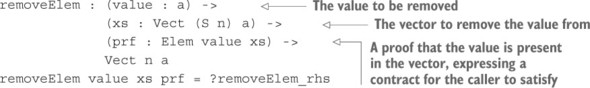
In type-driven development, we aim to use more-precise types to help direct the implementation of functions. Here, the input prf gives more precision to the input type of removeElem, and you can even case-split on it to see what you learn about the inputs value and xs from the relationship specified between them by prf.
You can write the function as follows:
- Define— Begin with the case split on prf:
removeElem : (value : a) -> (xs : Vect (S n) a) -> (prf : Elem value xs) -> Vect n a removeElem value (value :: ys) Here = ?removeElem_rhs_1 removeElem value (y :: ys) (There later) = ?removeElem_rhs_2
- Refine— For the first case, ?removeElem_rhs_1, you can see from the patterns that Idris has generated that value must be the first element in the vector if the proof has the form Here. You can therefore refine this case to remove value:
removeElem : (value : a) -> (xs : Vect (S n) a) -> (prf : Elem value xs) -> Vect n a removeElem value (value :: ys) Here = ys removeElem value (y :: ys) (There later) = ?removeElem_rhs_2
- Type— If you look at the type of ?removeElem_rhs_2, you’ll see that it appears you have the same problem as before, in that ys has length n, and removeElem requires a vector of length S n for the recursive call:
a : Type value : a y : a n : Nat ys : Vect n a later : Elem value ys -------------------------------------- removeElem_rhs_2 : Vect n a
But you have some further information that you didn’t have available earlier: you know from the variable later that value must occur in ys, and this means that ys must have a nonzero length. But how can you use this knowledge? - Define— Given that the length n must be nonzero, the trick is to case-split on n (by bringing it into scope using braces on the left side of the definition) and show that it’s impossible for it to be zero:
removeElem : (value : a) -> (xs : Vect (S n) a) -> (prf : Elem value xs) -> Vect n a removeElem value (value :: ys) Here = ys removeElem {n = Z} value (y :: ys) (There later) = ?removeElem_rhs_1 removeElem {n = (S k)} value (y :: ys) (There later) = ?removeElem_rhs_3 - Refine— Now, you can complete ?removeElem_rhs_3. You now know the length of ys is nonzero, so you can make a recursive call:
removeElem : (value : a) -> (xs : Vect (S n) a) -> (prf : Elem value xs) -> Vect n a removeElem value (value :: ys) Here = ys removeElem {n = Z} value (y :: ys) (There later) = ?removeElem_rhs_1 removeElem {n = (S k)} value (y :: ys) (There later) = y :: removeElem value ys laterNote that you need to pass later to the recursive call, as evidence that value is contained within ys. - Type, define—For the remaining hole, ?removeElem_rhs_1, take a look at its type and what variables are available:
a : Type value : a y : a ys : Vect 0 a later : Elem value ys -------------------------------------- removeElem_rhs_2 : Vect 0 a
You’re looking for an empty vector. That empty vector, if you look at the variables on the left side, should be a vector resulting from removing value from ys. This doesn’t make sense, because ys is an empty vector! You can make this more clear by case splitting on ys. Idris produces only one case:removeElem : (value : a) -> (xs : Vect (S n) a) -> (prf : Elem value xs) -> Vect n a removeElem value (value :: ys) Here = ys removeElem {n = Z} value (y :: []) (There later) = ?removeElem_rhs_1 removeElem {n = (S k)} value (y :: ys) (There later) = y :: removeElem value ys laterLooking at the type of the new hole, ?removeElem_rhs_1, shows the following:a : Type value : a y : a later : Elem value [] -------------------------------------- removeElem_rhs_1 : Vect 0 a
Previously, you’ve used the impossible keyword to rule out a case that doesn’t type-check. This case does type-check, so you can’t use impossible. But there’s no way you’ll ever have a value of type Elem value [] as an input, because there’s no way to construct an element of this type. - Refine— You can complete the definition using a function, absurd, defined in the Prelude. It has the following type:
absurd : Uninhabited t => t -> a
The Uninhabited interface, described in the sidebar, can be implemented for any type that has no values (as you saw with twoplustwo_not_five in chapter 8). So, you can refine ?remove_Elem_rhs_1 as follows:removeElem : (value : a) -> (xs : Vect (S n) a) -> (prf : Elem value xs) -> Vect n a removeElem value (value :: ys) Here = ys removeElem {n = Z} value (y :: []) (There later) = absurd later removeElem {n = (S k)} value (y :: ys) (There later) = y :: removeElem value ys later
interface Uninhabited t where uninhabited : t -> Void
There’s one method, which returns an element of the empty type. For example, you can provide an implementation of Uninhabited for 2 + 2 = 5:
Uninhabited (2 + 2 = 5) where uninhabited Refl impossible
Using uninhabited, the Prelude defines absurd as follows, using void:
absurd : Uninhabited t => (h : t) -> a absurd h = void (uninhabited h)
The additional argument to removeElem, of type Elem value xs, means that removeElem can work under the assumption that value is in the vector xs. It also means that you must provide a proof that value is in xs when calling the function.
9.1.4. auto-implicit arguments: automatically constructing proofs
If you try running removeElem with some specific values for the element and the vector, you’ll find you need to provide an additional argument for the proof. Sometimes it might be a proof that’s possible to construct:
*RemoveElem> removeElem 2 [1,2,3,4,5] removeElem 2 [1, 2, 3, 4, 5] : Elem 2 [1, 2, 3, 4, 5] -> Vect 4 Integer
Sometimes it might not:
*RemoveElem> removeElem 7 [1,2,3,4,5] removeElem 7 [1, 2, 3, 4, 5] : Elem 7 [1, 2, 3, 4, 5] -> Vect 4 Integer
In the first case, you can call removeElem by explicitly providing a proof of Elem 2 [1,2,3,4,5]:
*RemoveElem> removeElem 2 [1,2,3,4,5] (There Here) [1, 3, 4, 5] : Vect 4 Integer
The need to provide proofs explicitly like this can add a lot of noise to programs and can harm readability. Idris provides a special kind of implicit argument, marked with the keyword auto, to reduce this noise.
You can define a removeElem_auto function:
removeElem_auto : (value : a) -> (xs : Vect (S n) a) -> {auto prf : Elem value xs} -> Vect n a removeElem_auto value xs {prf} = removeElem value xs prf The third argument, named prf, is an auto-implicit argument. Like the implicit arguments you’ve already seen, an auto-implicit argument can be brought into scope by writing it in braces, and Idris will attempt to find a value automatically. Unlike ordinary implicits, Idris will search for a value for an auto implicit using the same machinery it uses for expression search with Ctrl-Alt-S in Atom. When you run removeElem_auto with arguments for value and xs, Idris will try to construct a proof for the argument marked auto:
*RemoveElem> removeElem_auto 2 [1,2,3,4,5] [1, 3, 4, 5] : Vect 4 Integer
If it can’t find a proof, it will report an error:
*RemoveElem> removeElem_auto 7 [1,2,3,4,5] (input):1:17:When checking argument prf to function Main.removeElem_auto: Can't find a value of type Elem 7 [1, 2, 3, 4, 5]
Alternatively, the following listing shows how you could define removeElem using an auto implicit directly.
Listing 9.3. Defining removeElem using an auto-implicit argument (RemoveElem.idr)
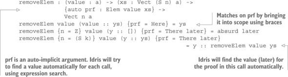
In general, though, you won’t know the specific values you’re passing to removeElem. They could be values read from a user or constructed by another part of the program. We’ll therefore need to consider how you can use removeElem when the inputs are unknown until runtime.
Just as you wrote a checkEqNat function to decide whether two numbers are equal, and later generalized it to decEq using an interface, you’ll need a function to decide whether a value is contained in a vector.
9.1.5. Decidable predicates: deciding membership of a vector
As you saw in the last chapter, a property is decidable if you can always say whether the property holds for some specific values. Using the following function, you can see that Elem value xs is a decidable property for specific values of value and xs, so Elem is a decidable predicate:
isElem : DecEq ty => (value : ty) -> (xs : Vect n ty) -> Dec (Elem value xs)
The type of isElem states that as long as you can decide equality of values in some type ty, you can decide whether a value with type ty is contained in a vector of types ty. Remember that Dec has the following constructors:
- Yes, which takes as its argument a proof that the predicate holds. In this case, that’s a value of type Elem value xs for whichever value and xs are passed as inputs to isElem.
- No, which takes as its argument a proof that the predicate doesn’t hold. In this case, that’s a value of type Elem value xs -> Void.
isElem is defined in Data.Vect, but it’s instructive to see how to write it yourself. The following listing shows our starting point, defining Elem by hand in a file named ElemType.idr.
Listing 9.4. Defining Elem and isElem by hand (ElemType.idr)
data Elem : a -> Vect k a -> Type where Here : Elem x (x :: xs) There : (later : Elem x xs) -> Elem x (y :: xs) isElem : DecEq a => (value : a) -> (xs : Vect n a) -> Dec (Elem value xs)
- Define, refine—Define the function by case splitting on the input vector xs:
isElem : DecEq a => (value : a) -> (xs : Vect n a) -> Dec (Elem value xs) isElem value [] = ?isElem_rhs_1 isElem value (x :: xs) = ?isElem_rhs_2
- Refine— For ?isElem_rhs_1, value is clearly not in the empty vector, so you can return No. Remember that No takes as an argument a proof that you can’t construct the predicate. You can leave a hole for this argument for the moment:
isElem : DecEq a => (value : a) -> (xs : Vect n a) -> Dec (Elem value xs) isElem value [] = No ?notInNil isElem value (x :: xs) = ?isElem_rhs_2
If you check the type of ?notInNil, you’ll see that to fill in this hole, you need to provide a proof that there can’t be an element of the empty vector:a : Type value : a constraint : DecEq a -------------------------------------- notInNil : Elem value [] -> Void
We’ll return to this hole shortly. - Refine— For ?isElem_rhs_2, if value and x are equal, you’ve found the value you’re looking for. You can use decEq, case-split on the result, and if the result is of the form Yes prf, return Yes with a hole for the proof that the value is the first in the vector:
isElem : DecEq a => (value : a) -> (xs : Vect n a) -> Dec (Elem value xs) isElem value [] = No ?notInNil isElem value (x :: xs) = case decEq value x of Yes prf => Yes ?isElem_rhs_1 No notHere => ?isElem_rhs_3
- Type, refine—You might like to fill the ?isElem_rhs_1 hole with Here, but if you check its type, you’ll see that you can’t quite use Here yet:
a : Type value : a x : a prf : value = x k : Nat xs : Vect k a constraint : DecEq a -------------------------------------- isElem_rhs_1 : Elem value (x :: xs)
You can’t use Here because the type you’re looking for isn’t of the form Elem value (value :: xs). But prf tells you that value and x must be the same, so if you case-split on prf, you’ll get this:isElem value (x :: xs) = case decEq value x of Yes Refl => Yes ?isElem_rhs_2 No notHere => ?isElem_rhs_3
The type of the newly created hole, ?isElem_rhs_2, is now in the form you need:a : Type value : a k : Nat xs : Vect k a constraint : DecEq a -------------------------------------- isElem_rhs_2 : Elem value (value :: xs)
You can fill in the ?isElem_rhs_2 using expression search in Atom:isElem : DecEq a => (value : a) -> (xs : Vect n a) -> Dec (Elem value xs) isElem value [] = No ?notInNil isElem value (x :: xs) = case decEq value x of Yes Refl => Yes Here No notHere => ?isElem_rhs_3
- Refine— For ?isElem_rhs_3, value and x aren’t equal (you know this because decEq value x has returned a proof), so you can search recursively in xs:
isElem : DecEq a => (value : a) -> (xs : Vect n a) -> Dec (Elem value xs) isElem value [] = No ?notInNil isElem value (x :: xs) = case decEq value x of Yes Refl => Yes Here No notHere => case isElem value xs of Yes prf => Yes ?isElem_rhs_1 No notThere => No ?isElem_rhs_2
Expression search will find the necessary proof for ?isElem_rhs_1. You can leave a hole for the No case for now:isElem : DecEq a => (value : a) -> (xs : Vect n a) -> Dec (Elem value xs) isElem value [] = No ?notInNil isElem value (x :: xs) = case decEq value x of Yes Refl => Yes Here No notHere => case isElem value xs of Yes prf => Yes (There prf) No notThere => No ?notInTail
At this stage, you can test the definition at the REPL. If a value is in a vector, you’ll see Yes and a proof:*ElemType> isElem 3 [1,2,3,4,5] Yes (There (There Here)) : Dec (Elem 3 [1, 2, 3, 4, 5])
If not, you’ll see No, with a hole for the proof that the element is missing:*ElemType> isElem 7 [1,2,3,4,5] No ?notInTail : Dec (Elem 7 [1, 2, 3, 4, 5])
To complete the definition, you’ll need to complete notInNil and notInTail. - Define, refine—You can complete ?notInNil by lifting it to a top-level function with Ctrl-Alt-L and then case splitting on its argument. Idris notices that neither input is possible:
notInNil : Elem value [] -> Void notInNil Here impossible notInNil (There _) impossible
- Define— You can complete ?notInTail similarly, but you’ll need to work a bit harder to show that each case is impossible. Lifting to a top-level definition and then case splitting on the argument leads to the following:
notInTail : (notThere : Elem value xs -> Void) -> (notHere : (value = x) -> Void) -> Elem value (x :: xs) -> Void notInTail notThere notHere Here = ?notInTail_rhs_1 notInTail notThere notHere (There later) = ?notInTail_rhs_2
For each hole, remember to check its type and the type of its local variables, because these will often give a strong hint as to how to proceed. - Refine— For each case, you can use either notHere or notThere to produce the value of type Void that you need:
notInTail : (notThere : Elem value xs -> Void) -> (notHere : (value = x) -> Void) -> Elem value (x :: xs) -> Void notInTail notThere notHere Here = notHere Refl notInTail notThere notHere (There later) = notThere later
Here’s the completed definition, for reference.
Listing 9.5. Complete definition of isElem (ElemType.idr)
notInNil : Elem value [] -> Void notInNil Here impossible notInNil (There _) impossible notInTail : (notThere : Elem value xs -> Void) -> (notHere : (value = x) -> Void) -> Elem value (x :: xs) -> Void notInTail notThere notHere Here = notHere Refl notInTail notThere notHere (There later) = notThere later isElem : DecEq a => (value : a) -> (xs : Vect n a) -> Dec (Elem value xs) isElem value [] = No notInNil isElem value (x :: xs) = case decEq value x of Yes Refl => Yes Here No notHere => case isElem value xs of Yes prf => Yes (There prf) No notThere => No (notInTail notThere notHere)
For comparison, listing 9.6 shows how you could define a Boolean test for checking vector membership. Here, I’ve used the Eq interface, so we don’t have any guarantees from the type about how the equality test behaves. Nevertheless, elem follows a structure similar to decElem.
Listing 9.6. A Boolean test for whether a value is in a vector (ElemBool.idr)
elem : Eq ty => (value : ty) -> (xs : Vect n ty) -> Bool elem value [] = False elem value (x :: xs) = case value == x of False => elem value xs True => True
Both definitions have a similar structure, but more work is required in isElem to show that the impossible cases are really impossible. As a trade-off, there’s no need for any tests for isElem, because the type is sufficiently precise that the implementation must be correct.
Exercises
- Data.List includes a version of Elem for List that works similarly to Elem for Vect. How would you define it?
- The following predicate states that a specific value is the last value in a List:
data Last : List a -> a -> Type where LastOne : Last [value] value LastCons : (prf : Last xs value) -> Last (x :: xs) value
So, for example, you can construct a proof of Last [1,2,3] 3:last123 : Last [1,2,3] 3 last123 = LastCons (LastCons LastOne)
Write an isLast function that decides whether a value is the last element in a List. It should have the following type:isLast : DecEq a => (xs : List a) -> (value : a) -> Dec (Last xs value)
You can test your answer at the REPL as follows:*ex_9_1> isLast [1,2,3] 3 Yes (LastCons (LastCons LastOne)) : Dec (Last [1, 2, 3] 3)
9.2. Expressing program state in types: a guessing game
In practice, the need for predicates like Elem and functions like removeElem arises naturally when we write functions that express characteristics of system state, such as vector length, in their types. To conclude this chapter, we’ll look at a small example of where this happens: using the type system to encode simple properties of a word-guessing game, Hangman.
In Hangman, a player tries to guess a word by guessing one letter at a time. If they guess all the letters in the word, they win. Otherwise, they’re allowed a limited number of incorrect guesses, after which they lose.
9.2.1. Representing the game’s state
Listing 9.7 shows how we can represent the current state of a word game as a data type, WordState, in Idris. There are two important parts of the state that capture the features of the game, and they’re written as parts of the type:
- The number of guesses the player has remaining
- The number of letters the player still has to guess
Listing 9.7. The game state (Hangman.idr)
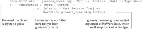
A game is finished if either the number of guesses remaining is zero (in which case the player has lost) or the number of letters remaining is zero (in which case the player has won). Listing 9.8 shows how we can represent this in a data type. We can be certain that this captures only games that are won or lost, because we’re including the number of guesses and the number of letters remaining as arguments to WordState.
Listing 9.8. Defining precisely when a game is in a finished state (Hangman.idr)
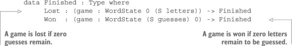
9.2.2. A top-level game function
We’ll take a top-down approach, defining a top-level function that implements a complete game. The following listing gives the starting point.
Listing 9.9. Top-level game function (Hangman.idr)

The type of game states that a game can proceed if there’s at least one guess remaining (S guesses) and at least one letter still to guess (S letters). It returns IO Finished, meaning that it performs interactive actions that produce game data in a Finished state.
To implement the game, you’ll need to read a single letter from the user (any other input is invalid), check whether the letter input by the user is in the target word in the game state, update the game state, and loop if the game isn’t complete. You can update the state in one of the following ways:
- The letter is in the word, in which case you continue the game with the same number of guesses and one fewer letter.
- The letter isn’t in the word, in which case you continue the game with one fewer guess and the same number of letters.
The numbers of guesses and letters used and remaining are explicitly recorded in the game state’s type. The next step, therefore, is to write a function that captures these state updates in its type.
9.2.3. A predicate for validating user input: ValidInput
You can read user input using the IO action getLine:
getLine : IO StringBut because the user is guessing a letter, the only inputs that are valid are those that consist of exactly one character. For precision, you can make the notion of a valid input explicit in a predicate. Because String is a primitive, it’s difficult to reason about its individual components in a type, so you can use a List Char to represent the input in the predicate and convert as necessary:
data ValidInput : List Char -> Type where Letter : (c : Char) -> ValidInput [c]
To check whether a String is a valid input, you can write the following function, which returns either a proof that the input is valid, or a proof that it can never be valid, using Dec:
isValidString : (s : String) -> Dec (ValidInput (unpack s))
You’ll see the definition of isValidString shortly, in section 9.2.5. As an exercise, you can try writing it yourself, beginning with the following helper function:
isValidInput : (cs : List Char) -> Dec (ValidInput cs)
Then, instead of using getLine, write a readGuess function that returns the user’s guess, along with an instance of a predicate that guarantees the user’s guess is a valid input:
readGuess : IO (x ** ValidInput x)
readGuess returns a dependent pair, where the first element is the input read from the console, and the second is a predicate that the input must satisfy.
Contracts on return values
By returning a value paired with a predicate on that value, the type of readGuess is expressing a contract that the return value must satisfy.
The following listing gives the definition of readGuess.
Listing 9.10. Read a guess from the console, which is guaranteed to be valid (Hangman.idr)
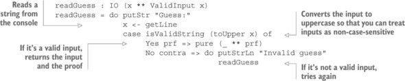
By using readGuess, you can be certain that any valid string read from the console is guaranteed to contain exactly one character.
9.2.4. Processing a guess
Processing a guess will return a game state with one type if the guess is correct, and a different type if the guess is incorrect. You can use the Either generic type to represent this. Remember that Either is a generic type defined in the Prelude that carries a value of two possible types:data Either a b = Left a | Right b
Either is often used to represent the result of a computation that might fail, carrying information about the error if it does fail. By convention, we use Left for the error case and Right for the success case.[1] You can think of an incorrect guess as being the error case, so the next listing shows the type you’ll use for a function that processes a guess.
“Right” also being a synonym of “correct.”
1
Listing 9.11. Type of a function that processes a user’s guess (Hangman.idr)
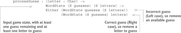
This type states that, given a letter and an input game state, it will either produce a new game state where the number of guesses remaining has decreased (the guess was incorrect), or where the number of letters remaining has decreased (the guess was correct.)
Types as abstract state
A value of type WordState guesses letters holds concrete information about system state, including the exact word to be guessed and exactly which letters are still missing. The type itself expresses abstract information about the game state (guesses remaining and number of missing letters), which allows you to express the rules in function types like processGuess.
You can implement processGuess as follows:
- Define— You need to inspect the input game state, so you can case-split on the input state:
processGuess : (letter : Char) -> WordState (S guesses) (S letters) -> Either (WordState guesses (S letters)) (WordState (S guesses) letters) processGuess letter (MkWordState word missing) = ?guess_rhs_1
- Define— If the guessed letter is correct, it’ll be in the missing vector, and you’ll need to remove it. You can use isElem to find whether it’s there and define the function by case splitting on the result of isElem:
processGuess letter (MkWordState word missing) = case isElem letter missing of Yes prf => ?guess_rhs_2 No contra => ?guess_rhs_3
- Refine— If the letter is in the vector of missing letters, you’ll return a new state with one fewer letters to guess. Otherwise, you’ll return a new state with one fewer guess available:
processGuess letter (MkWordState word missing) = case isElem letter missing of Yes prf => Right (MkWordState word ?nextVect) No contra => Left (MkWordState word missing)
You have a hole, ?nextVect, for the updated vector of missing letters. - Type, refine—The type of ?nextVect shows that you need to remove an element from the vector:
word : String letter : Char letters : Nat missing : Vect (S letters) Char prf : Elem letter missing guesses : Nat -------------------------------------- nextVect : Vect letters Char
You can complete the definition by using removeElem to remove letter from missing, and Idris will find the necessary proof, prf, as an auto implicit. This completes the definition:processGuess : (letter : Char) -> WordState (S guesses) (S letters) -> Either (WordState guesses (S letters)) (WordState (S guesses) letters) processGuess letter (MkWordState word missing) = case isElem letter missing of Yes prf => Right (MkWordState word (removeElem letter missing)) No contra => Left (MkWordState word missing)
Explicit assumptions
In the game state, you assume that the number of letters still to guess is the same as the length of the vector of missing letters. By putting this in the type of WordState and the type of processGuess, you can be sure that if you ever violate this assumption, your program will no longer compile.
You can complete the definition of game using processGuess to update the game state as necessary.
9.2.5. Deciding input validity: checking ValidInput
Before completing the implementation of game, you’ll need to complete your implementation of isValidString, which decides whether a string entered by the user is a valid input or not.Listing 9.12. Showing that an input string must be either a valid or invalid input (Hangman.idr)
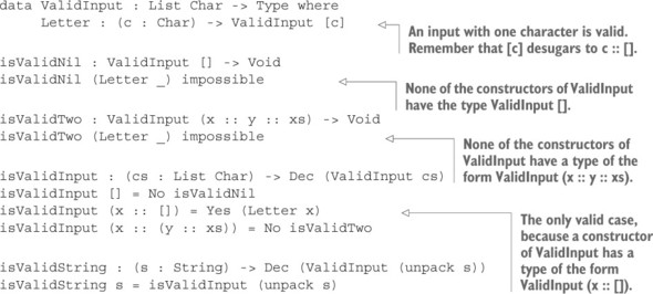
You can test this definition at the REPL by using >>= to take the output of read-Guess, matching on the first component of the dependent pair, and passing it on to printLn:
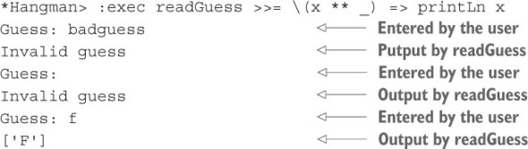
Now that you have the ability to read input that’s guaranteed to be in a valid form, and the ability to process guesses to update the game state, you can complete the top-level game implementation.
9.2.6. Completing the top-level game implementation
The next listing shows one possible (if basic) way to complete the implementation of game. It uses processGuess to check the user’s input and reports whether a guess is correct or incorrect until the player has won or lost.
Listing 9.13. Top-level game function (Hangman.idr)
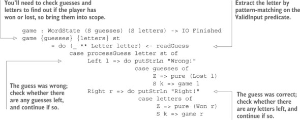
- It’s impossible to test the wrong variable (guesses or letters) before continuing the game.[2] Doing so would cause a type error.
I really did make this mistake when writing this example!2 - It’s impossible to continue a completed game, because there must be at least one guess remaining and at least one letter to guess.
- It’s impossible to finish a game prematurely, when there are both missing letters and guesses still available.
The following listing shows a possible implementation of main that sets up a game with a target word, "Test", so requiring a player to guess the letters 'T', 'E', and 'S'.
Listing 9.14. A main program to set up a game (Hangman.idr)
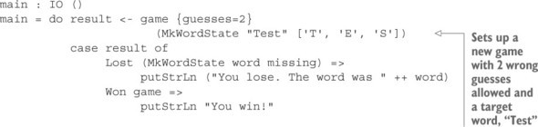
9.3. Summary
- You can write types that express assumptions about how values relate.
- The Elem dependent type is a predicate that expresses that a value must be contained in a vector.
- By passing a predicate as an argument to a function, you can express a contract that the inputs to the function must follow.
- You can write a function to show that a predicate is decidable, using Dec.
- Idris will attempt to find values for arguments marked auto by expression search.
- You can capture properties of a system’s state (such as the rules of a game) in a type.
- Predicates can describe the validity of user input and ensure that the user input is validated when necessary.
Chapter 10. Views: extending pattern matching
This chapter covers
- Defining views, which describe alternative forms of pattern matching
- Introducing the with construct for working with views
- Describing efficient traversals of data structures
- Hiding the representation of data behind views
In type-driven development, our approach to implementing functions is to write a type, define the structure of the function by case splits on its arguments, and refine the function by filling in holes. In the define step in particular, we use the structure of the input types to drive the structure of the function as a whole.
As you learned in chapter 3, when you case-split on a variable, the patterns arise from the variable’s type. Specifically, the patterns arise from the data constructors that can be used to build values of that type. For example, if you case-split on an items variable of type List elem, the following patterns will arise:
- []—Represents the empty list
- (x :: xs)—Represents a non-empty list with x as the first element and xs as the list of the remaining elements
- A list of all but the last element, and then the last element
- Two sublists—the first half and the second half of the input
In this chapter, you’ll see how to extend the forms of patterns you can use by defining informative data types, called views. Views are dependent types that are parameterized by the data you’d like to match, and they give you new ways of observing that data. For example, views can do the following:
- Describe new forms of patterns, such as allowing you to match against the last element of a list rather than the first
- Define alternative ways of traversing data structures, such as traversing a list in reverse, or by repeatedly splitting the list into halves
- Hide complex data representations behind an abstract interface while still supporting pattern-matching on that data
We’ll start by looking at how, using views, we can define alternative ways of matching on lists, such as processing the last element first. We’ll then look at defining efficient traversals of lists and guaranteeing that they terminate, and we’ll look at some traversals provided by the Idris library. Finally, we’ll use views to help with data abstraction by hiding the structure of data in a separate module and matching and traversing the data using a view.
10.1. Defining and using views
When you write a (x :: xs) pattern for matching a list, x will take the value of the first element of the list and xs will take the value of the tail of the list. You saw the following function in chapter 3 to describe how a list was constructed, illustrated again in figure 10.1:
describeList : List Int -> String describeList [] = "Empty" describeList (x :: xs) = "Non-empty, tail = " ++ show xs
Figure 10.1. Matching the pattern (x :: xs) for inputs [1] and [2,3,4,5]
You can add a single element to the end of a list using the ++ operator:
Idris> [2,3,4] ++ [5] [2, 3, 4, 5] : List Integer
It would be nice to be able to match patterns of the form (xs ++ [x]), where x takes the value of the last element of the list and xs takes the value of the initial segment of the list. That is, you might like to be able to write a function of the following form, as illustrated in figure 10.2:

Figure 10.2. Matching the pattern (xs ++ [x]) for inputs [1] and [2,3,4,5]
Unfortunately, if you try to implement describeListEnd, it will fail with the following error:
DLFail.idr:3:19: When checking left hand side of describeListEnd: Can't match on describeListEnd (xs ++ [x])
The problem is that you’re trying to pattern-match on the result of a function, ++, and in general there’s no way for Idris to automatically deduce the inputs to an arbitrary function from its output. You can, however, extend the forms of the patterns you can use by defining informative data types called views. In this section, you’ll see how to define views, and I’ll introduce the with construct, which provides a concise notation for defining functions that use views.
10.1.1. Matching the last item in a list
You can’t write describeListEnd directly because you can’t match a pattern of the form (xs ++ [x]) directly. You can, however, take advantage of dependent pattern matching to deduce that a particular input must have the form (xs ++ [x]). You saw
dependent pattern matching in chapter 6, where inspecting the value of one argument (that is, case-splitting on that argument) can tell you about the form of another. Using dependent pattern matching, you can describe alternative patterns for lists.The following listing shows the ListLast dependent type, which describes two possible forms a List can take. A list is either empty, [], or constructed from the initial portion of a list and its final element.
Listing 10.1. The ListLast dependent type, which gives alternative patterns for a list (DescribeList.idr)
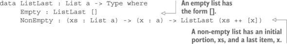
Using ListLast, along with dependent pattern matching, you can define describe-ListEnd. You’ll start by defining a helper function that takes an input list, input, and an extra argument, form, that says whether the list is empty or non-empty:
- Type— Begin with the type. You’ll use ListLast to describe the possible forms that input can take:
describeHelper : (input : List Int) -> (form : ListLast input) -> String describeHelper input form = ?describeHelper_rhs
- Define— You want to describe input, so you’ll need to inspect its form somehow. Previously, when defining a function to inspect the form of an input, you’ve case-split on that input. Here, the intention of the form argument is to tell you more about input, so case-split on that instead:
describeHelper : (input : List Int) -> (form : ListLast input) -> String describeHelper [] Empty = ?describeHelper_rhs_1 describeHelper (xs ++ [x]) (NonEmpty xs x) = ?describeHelper_rhs_2
Notice that the case split on form has told you more about the form of input. In particular, the type of NonEmpty means that if form has the value NonEmpty xs x, then input must have the value (xs ++ [x]). - Refine— Complete the definition by describing the patterns as in our initial attempt at describeListEnd:
describeHelper : (input : List Int) -> ListLast input -> String describeHelper [] Empty = "Empty" describeHelper (xs ++ [x]) (NonEmpty xs x) = "Non-empty, initial portion = " ++ show xs
ListLast is a view of lists because it provides an alternative means of viewing the data. It’s an ordinary data type, though, and in order to use ListLast in practice, you’ll need to be able to convert an input list, xs, into a value of type ListLast xs.
10.1.2. Building views: covering functions
The next listing shows listLast, which converts an input list, xs, into an instance of a view, ListLast xs, which gives access to the last element of xs.Listing 10.2. Describing a List in the form ListLast (DescribeList.idr)
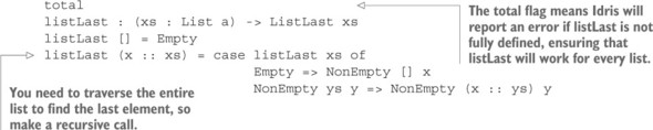
listLast is the covering function of the ListLast view. A covering function of a view describes how to convert a value (in this case the input list) into a view of that value (in this case, an xs list and a value x, where xs ++ [x] = input).
Naming convention for covering functions
By convention, covering functions are given the same name as the view type, but with an initial lowercase letter.
Now that you can describe any List in the form ListLast, you can complete the definition of describeListEnd:
describeHelper : (input : List Int) -> ListLast input -> String describeHelper [] Empty = "Empty" describeHelper (xs ++ [x]) (NonEmpty xs x) = "Non-empty, initial portion = " ++ show xs describeListEnd : List Int -> String describeListEnd xs = describeHelper xs (listLast xs)
This works as we intended in our initial attempt at describeListEnd, with the original patterns in describeHelper. Given that you’re using a different notion of pattern matching than the default, you should expect to have to use some additional notation to explain how to match the pattern (xs ++ [x]), but the overall definition still feels quite verbose.
Because dependent pattern matching in this way is a common programming idiom in Idris, there’s a construct for expressing extended pattern matching more concisely: the with construct.
10.1.3. with blocks: syntax for extended pattern matching
Using views to generate informative patterns like (xs ++ [x]) can help the readability of functions and increase your confidence in their correctness because the types tell you exactly what form the inputs must take. But these functions can be a little more verbose because you need to create an extra helper function (like describeHelper) to
do the necessary pattern matching. The with construct provides a notation for using views more concisely.Using with blocks, you can add extra arguments to the left side of a definition, giving you more arguments to case-split. The easiest way to see how this works is by example, so let’s take a look at how you can use a with block to define describeListEnd:
- Type— Begin with a top-level type that takes a List Int and returns a String:
describeListEnd : List Int -> String describeListEnd input = ?describeListEnd_rhs
- Define— Press Ctrl-Alt-W with the cursor on the line with the hole ?describe-ListEnd_rhs. This adds a new pattern clause as follows (it won’t yet type-check):
describeListEnd : List Int -> String describeListEnd input with (_) describeListEnd input | with_pat = ?describeListEnd_rhs
- Define— The with syntax adds a new argument to the left side of the definition. The brackets after with give the value of that argument, and the (indented) clause beneath contains the extra argument, after a vertical bar. Here, you’ll match on the result of listLast input, so replace the _ with listLast input:
describeListEnd : List Int -> String describeListEnd input with (listLast input) describeListEnd input | with_pat = ?describeListEnd_rhs
- Type— If you check the type of ?describeListEnd_rhs, you can see more detail about how with works, looking specifically at the type of with_pat:
input : List Int with_pat : ListLast input -------------------------------------- describeListEnd_rhs : String
The value of with_pat is the result of listLast input. Figure 10.3 shows the components of the syntax for the with construct. Note that the scope of the with block is managed by indentation.Figure 10.3. Syntax for the with construct
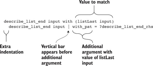
- Define— Notice that the types of input and with_pat are exactly the same as the types of the inputs to describeHelper earlier. And as in the definition of describeHelper, if you case-split on with_pat, you’ll learn more about the form of input:
describeListEnd : List Int -> String describeListEnd input with (listLast input) describeListEnd [] | Empty = ?describeListEnd_rhs_1 describeListEnd (xs ++ [x]) | (NonEmpty xs x) = ?describeListEnd_rhs_2
- Refine— Complete the definition as before, with the description of the patterns:
describeListEnd : List Int -> String describeListEnd input with (listLast input) describeListEnd [] | Empty = "Empty" describeListEnd (xs ++ [x]) | (NonEmpty xs x) = "Non-empty, initial portion = " ++ show xs
Effectively, the with construct has allowed you to use an intermediate pattern match, on the result of listLast input, without needing to define a separate function like describeHelper. In turn, matching on the result of listLast input gives you more-informative patterns for input.
The difference between with and case
The purpose of the with construct is similar to that of a case block in that it allows matching on intermediate results. There’s one important difference, however: with introduces a new pattern to match on the left side of a definition. As a result, you can use dependent pattern matching directly. In describeListEnd, for example, matching on the result of listLast input told you about the form input must take.
You can’t use just any expression in a pattern because it isn’t possible, in general, to decide what the inputs to a function must be, given only its result. Idris therefore allows patterns only when it can deduce those inputs, which is in the following cases:
- The pattern consists of a data constructor applied to some arguments. The arguments must also be valid patterns.
- The value of the pattern is forced by some other valid pattern. In the case of describeListEnd, the value of the pattern (xs ++ [x]) is forced by the valid pattern NonEmpty xs x.
10.1.4. Example: reversing a list using a view
Once you have the ability to pattern-match in different ways using views, you can traverse data structures in new ways. Rather than always traversing a list from left to right, for example, you can use listLast to traverse a list from right to left, inspecting the last element first.
You can reverse a list in this way:
- To reverse an empty list [], return [].
- To reverse a list in the form xs ++ [x], reverse xs and then add x to the front of the list.
- Type— Call the function myReverse because there’s already a reverse function in the Prelude:
myReverse : List a -> List a myReverse input = ?myReverse_rhs
- Define— You’ll define the function by inspecting the last element of the input first, so you can use listLast to match on a value of type ListLast input. Press Ctrl-Alt-W to insert a with block, and add listLast input as the value to inspect:
myReverse : List a -> List a myReverse input with (listLast input) myReverse input | with_pat = ?myReverse_rhs
- Define— Next, case-split on with_pat to give the relevant patterns for input:
myReverse : List a -> List a myReverse input with (listLast input) myReverse [] | Empty = ?myReverse_rhs_1 myReverse (xs ++ [x]) | (NonEmpty xs x) = ?myReverse_rhs_2
- Refine— Finally, you can complete the definition as follows:
myReverse : List a -> List a myReverse input with (listLast input) myReverse [] | Empty = [] myReverse (xs ++ [x]) | (NonEmpty xs x) = x :: myReverse xs
This is a fairly direct implementation of the algorithm, traversing the list in reverse and constructing a new list by adding the last item of the input as the first item of the result. There are, nevertheless, two problems:
- The definition is inefficient because it constructs ListLast input on every recursive call, and constructing ListLast input requires traversing input.
- Idris can’t decide whether the definition is total or not:
*Reverse> :total myReverse Main.myReverse is possibly not total due to: possibly not total due to recursive path: with block in Main.myReverse, with block in Main.myReverse
See the sidebar for a brief discussion on totality checking in Idris.
The first problem is important to address, because it’s possible to write myReverse in linear time, traversing the input list only once. The second problem is important from the type-driven development perspective: as I discussed in chapter 1, if Idris can determine that a function is total, you have a strong guarantee that the type accurately describes what the function will do. If not, you only have a guarantee that the function will produce a value of the given type if it terminates without crashing. Furthermore, if Idris can’t determine that a function is total, it can’t determine that any functions that call it are total, either.
We’ll look at how to address each of these problems, with only minor alterations to myReverse itself, in section 10.2.Idris tries to decide whether a function is always terminating by checking two things:
- There must be patterns for all possible well-typed inputs.
- When there is a recursive call (or a sequence of mutually recursive calls), there must be a decreasing argument that converges toward a base case.
To determine which arguments are decreasing, Idris looks at the patterns for the inputs in a definition. If a pattern is in the form of a data constructor, Idris considers the arguments in that pattern to be smaller than the input. In myReverse, for example, Idris doesn’t consider xs to be smaller than (xs ++ [x]), because (xs ++ [x]) is not in the form of a data constructor.
This restriction keeps the concept of decreasing argument simple for Idris to check. In general, Idris can’t tell whether the inputs to a function will always be smaller than the result.
As you’ll see in section 10.2, you can work around this restriction by defining recursive views.
10.1.5. Example: merge sort
Views allow you to describe matching on data structures any way you like, with as many patterns as you like, provided you can implement a covering function for the view. As a second example of a view, we’ll implement the merge sort algorithm on Lists.
Merge sort, at a high level, works as follows:
- If the input is an empty list, return an empty list.
- If the input has one element, it’s already sorted, so return the input.
- In all other cases, split the list into two halves (differing in size by at most one), recursively sort those halves, and then merge the two sorted halves into a sorted list (see figure 10.4).
Figure 10.4. Sorting a list using merge sort: split the list into two halves, sort the halves, and then merge the sorted halves back together
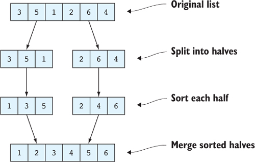
Idris> :doc merge Prelude.List.merge : Ord a => List a -> List a -> List a Merge two sorted lists using the default ordering for the type of their elements.
Note that it has a generic type and requires the Ord interface to be implemented for the element type of the list.
Assuming that the two input lists are sorted, merge will produce a sorted list of the elements in the input lists. For example, the lists in figure 10.4 would be merged as follows:
Idris> merge [1,3,5] [2,4,6] [1, 2, 3, 4, 5, 6] : List Integer
Listing 10.3 shows how you might ideally like to write a mergeSort function that sorts a list using the merge sort algorithm. Unfortunately, as it stands, this won’t work because (lefts ++ rights) isn’t a valid pattern.
Listing 10.3. Initial attempt at mergeSort with an invalid pattern (MergeSort.idr)
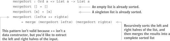
Given an input list matched against a pattern, (lefts ++ rights), Idris can’t in general deduce what lefts and rights must be; indeed, there could be several reasonable possibilities if the input list has one or more elements. Here are a couple of examples:
- [1] could match against (lefts ++ rights) with lefts as [1] and rights as [], or lefts as [] and rights as [1].
- [1,2,3] could match against (lefts ++ rights) with lefts as [1] and rights as [2,3], or lefts as [1,2] and rights as [3], among many other possibilities.
To match the patterns we want, as shown in listing 10.3, you’ll need to create a view of lists, SplitList, that gives the patterns you want. The following listing shows the definition of SplitList and gives the type for its covering function, splitList.
Listing 10.4. A view of lists that gives patterns for empty lists, singleton lists, and concatenating lists (MergeSort.idr)
data SplitList : List a -> Type where SplitNil : SplitList [] SplitOne : SplitList [x] SplitPair : (lefts : List a) -> (rights : List a) -> SplitList (lefts ++ rights) splitList : (input : List a) -> SplitList input
I’ll give a definition of the covering function, splitList, shortly. For now, note that as long as the implementation of splitList is total, you can be sure from its type that it gives valid patterns for empty lists, singleton lists, or concatenations of two lists. You don’t, however, have any guarantees in the type about how a list is split into pairs; in this case, you need to rely on the implementation to ensure that lefts and rights differ in size by at most one.
Precision of SplitPair
In principle, you could make the type of SplitPair more precise and carry a proof that lefts and rights differ in size by at most one. In fact, the Idris library module Data.List.Views exports such a view, called SplitBalanced.
You can implement mergeSort using the SplitList view as follows:
- Type— Begin with the type and a skeleton definition:
mergeSort : Ord a => List a -> List a mergeSort input = ?mergeSort_rhs
- Define— To get the patterns you want, you’ll need to use the SplitList view you’ve just created. Add a with block and use the splitList covering function:
mergeSort : Ord a => List a -> List a mergeSort input with (splitList input) mergeSort input | with_pat = ?mergeSort_rhs
- Define— If you case-split on with_pat, you’ll get appropriate patterns for input arising from the types of the constructors to SplitList:
mergeSort : Ord a => List a -> List a mergeSort input with (splitList input) mergeSort [] | SplitNil = ?mergeSort_rhs_1 mergeSort [x] | SplitOne = ?mergeSort_rhs_2 mergeSort (lefts ++ rights) | (SplitPair lefts rights) = ?mergeSort_rhs_3
- Refine— You can complete the definition by filling in the right sides for each pattern, directly following the high-level description of the merge sort algorithm I gave at the start of this section:
mergeSort : Ord a => List a -> List a mergeSort input with (splitList input) mergeSort [] | SplitNil = [] mergeSort [x] | SplitOne = [x] mergeSort (lefts ++ rights) | (SplitPair lefts rights) = merge (mergeSort lefts) (mergeSort rights)
Listing 10.5. Defining a covering function for SplitList (MergeSort.idr)
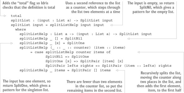
You build two (approximately) equally sized lists by using a second reference to the input list as a counter in a helper function, splitListHelp, as follows:
- On each recursive call, the counter steps through two elements of the list. The pattern (_ :: _ :: counter) matches any list with at least two elements, where counter is a list containing all but the first two elements.
- When the counter reaches the end of the list (that is, fewer than two elements remain), you must have traversed half of the input.
You can now try splitList and mergeSort at the REPL:
*MergeSort> splitList [1] SplitOne : SplitList [1] *MergeSort> splitList [1,2,3,4,5] SplitPair [1, 2] [3, 4, 5] : SplitList [1, 2, 3, 4, 5] *MergeSort> mergeSort [3,2,1] [1, 2, 3] : List Integer *MergeSort> mergeSort [5,1,4,3,2,6,8,7,9] [1, 2, 3, 4, 5, 6, 7, 8, 9] : List IntegerBy defining a view that gives possible cases for the input list in terms of how it can be split in half, you can write a definition of mergeSort that directly implements the high-level description of the algorithm.
Like myReverse, however, Idris can’t tell whether mergeSort is total:
*MergeSort> :total mergeSort Main.mergeSort is possibly not total due to: possibly not total due to recursive path: with block in Main.mergeSort, with block in Main.mergeSort
Again, the problem is that Idris can’t tell that the recursive calls are guaranteed to be on smaller lists than the original input. In the next section, you’ll see how to address this problem by defining recursive views that describe the recursive structure of a function, as well as the patterns that define a function.
Exercises
- The TakeN view allows traversal of a list several elements at a time:
data TakeN : List a -> Type where Fewer : TakeN xs Exact : (n_xs : List a) -> TakeN (n_xs ++ rest) takeN : (n : Nat) -> (xs : List a) -> TakeN xs
The Fewer constructor covers the case where there are fewer than n elements. Define the covering function takeN. To check that your definition works, you should be able to run the following function, which groups lists into sublists with n elements each:groupByN : (n : Nat) -> (xs : List a) -> List (List a) groupByN n xs with (takeN n xs) groupByN n xs | Fewer = [xs] groupByN n (n_xs ++ rest) | (Exact n_xs) = n_xs :: groupByN n rest
Here’s an example:*ex_10_1> groupByN 3 [1..10] [[1, 2, 3], [4, 5, 6], [7, 8, 9], [10]] : List (List Integer)
- Use TakeN to define a function that splits a list into two halves by calculating its length:
halves : List a -> (List a, List a)
If you have implemented this correctly, you should see the following:*ex_10_1> halves [1..10] ([1, 2, 3, 4, 5], [6, 7, 8, 9, 10]) : (List Integer, List Integer) *ex_10_1> halves [1] ([], [1]) : (List Integer, List Integer)
Hint: Use div for dividing a Nat.
10.2. Recursive views: termination and efficiency
The purpose of views is to give us new ways to match on data, using the with construct for a more concise syntax. When you write a function with a view, you use the following components:- The original input data
- A view of the input data, where the view data type is parameterized by the input data
- A covering function for the view, which constructs an instance of the view for the input data
Then, using the with construct, you can pattern-match on the view. Dependent pattern matching gives you informative patterns for the original data. You’ve seen two examples of this in the previous section: reversing a list, and splitting a list in half for merge sort. In both cases, however, Idris couldn’t tell that the resulting function was total. Moreover, when you reverse a list, the resulting function is inefficient because it has to reconstruct the view on every recursive call.
In this section, we’ll look at how to solve both these problems by defining recursive views for describing traversals of data structures. Furthermore, once we’ve defined a view, we can reuse it for any function that uses the same recursion pattern. The Idris library provides a number of useful views for traversals of data structures, and we’ll look at some example functions with some of these. First, though, we’ll improve the definition of myReverse.
10.2.1. “Snoc” lists: traversing a list in reverse
A snoc list is a list where elements are added to the end of the list, rather than the beginning. We can define them as follows, as a generic data type:
data SnocList ty = Empty | Snoc (SnocList ty) ty
Snoc list terminology
The name snoc list arises because the traditional name (originating with Lisp) for the operator that adds an element to the beginning of a list is cons. Therefore, the name for the operator that adds an element to the end of a list is snoc.
Using SnocList, you traverse the elements in reverse order, because the element (of type ty) appears after the list (of type SnocList ty). You can easily produce a List from a SnocList where the elements are in reverse order:
reverseSnoc : SnocList ty -> List ty reverseSnoc Empty = [] reverseSnoc (Snoc xs x) = x :: reverseSnoc xs
You can show the relationship between SnocList and List more precisely by parameterizing SnocList over the equivalent List. The following listing shows how to define SnocList in this way.
Listing 10.6. The SnocList type, parameterized over the equivalent List (SnocList.idr)
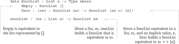
Here, SnocList is a recursive view, and snocList is its covering function. We’ll come to the definition of snocList shortly; first, let’s see how you can use this to implement myReverse:
- Type— Begin by defining a helper function that takes a list, input, and its equivalent SnocList:
myReverseHelper : (input : List a) -> SnocList input -> List a myReverseHelper input snoc = ?myReverseHelper_rhs
- Define— If you case-split on snoc, you’ll get corresponding patterns for input:
myReverseHelper : (input : List a) -> SnocList input -> List a myReverseHelper [] Empty = ?myReverseHelper_rhs_1 myReverseHelper (xs ++ [x]) (Snoc rec) = ?myReverseHelper_rhs_2
- Refine— If the input is empty, you’ll return the empty list:
myReverseHelper : (input : List a) -> SnocList input -> List a myReverseHelper [] Empty = [] myReverseHelper (xs ++ [x]) (Snoc rec) = ?myReverseHelper_rhs_2
- Refine, type— Otherwise, you’ll recursively reverse xs and add the item x to the front:
myReverseHelper : (input : List a) -> SnocList input -> List a myReverseHelper [] Empty = [] myReverseHelper (xs ++ [x]) (Snoc rec) = x :: myReverseHelper xs ?snocrec
There’s still a hole, ?snocrec, for the second argument in the recursive call. If you inspect it, you’ll see that you need the SnocList that represents xs:a : Type xs : List a rec : SnocList xs x : a -------------------------------------- snocrec : SnocList xs
- Refine— Fortunately, you already have a value, rec, of type SnocList xs, so you can use it directly to complete the definition:
myReverseHelper : (input : List a) -> SnocList input -> List a myReverseHelper [] Empty = [] myReverseHelper (xs ++ [x]) (Snoc rec) = x :: myReverseHelper xs rec
- Define— Finally, you can define myReverse by building a SnocList and calling myReverseHelper:
myReverse : List a -> List a myReverse input = myReverseHelper input (snocList input)
You can’t test this yet because you haven’t implemented snocList, but for now notice how this contrasts with the implementation of myReverse in section 10.1.4, using ListLast. The similarity is that you find the patterns for the input list by matching on a view of input. The difference is that the view is recursive, meaning that you don’t have to rebuild the view on each recursive call; you already have access to it.
The definition of myReverseHelper is total, because the SnocList argument is decreasing on each recursive call:
*SnocList> :total myReverseHelper Main.myReverseHelper is Total
It now remains to implement snocList. As long as you can implement snocList by traversing the list only once, you’ll have an implementation of myReverse that runs in linear time. The following listing shows an implementation of snocList that traverses the list only once, using a helper function with an accumulator to build the SnocList by adding one element at a time.
Listing 10.7. Implementing the covering function snocList
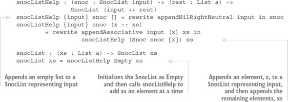
The definition of snocList is slightly tricky, involving the rewrite construct (which you saw in chapter 8) to get the types in the correct form for building the SnocList. You’ll rewrite with the following functions from the Prelude:
appendNilRightNeutral : (l : List a) -> l ++ [] = l appendAssociative : (l : List a) -> (c : List a) -> (r : List a) -> l ++ (c ++ r) = (l ++ c) ++ rAs with any complex definition, it’s a good idea to try to understand it by replacing subexpressions of the definition with holes, and seeing what the types of those holes are. In this case, it’s also useful to remove the rewrite constructs and replace them with holes, to see how the types need rewriting:
snocListHelp : SnocList input -> (xs : List a) -> SnocList (input ++ xs) snocListHelp {input} snoc [] = ?rewriteNil snoc snocListHelp {input} snoc (x :: xs) = ?rewriteCons (snocListHelp (Snoc snoc {x}) xs) You should see the following types for rewriteNil and rewriteCons:
rewriteNil : SnocList input -> SnocList (input ++ []) rewriteCons : SnocList ((input ++ [x]) ++ xs) -> SnocList (input ++ x :: xs)
The good news is that once you’ve defined snocList, you can reuse it for any function that needs to traverse a list in reverse. Furthermore, as you’ll see shortly, a SnocList view is also defined in the Idris library, along with several others.
10.2.2. Recursive views and the with construct
You now have an implementation of myReverse that runs in linear time, because it traverses the list once to build the SnocList view and then traverses the SnocList view once to build the reversed list. You can also confirm that Idris believes it’s total:
*SnocList> :total myReverse Main.myReverse is Total
The resulting definition isn’t quite as concise as the previous definition of myReverse, however, because it doesn’t use the with construct:
myReverseHelper : (input : List a) -> SnocList input -> List a myReverseHelper [] Empty = [] myReverseHelper (xs ++ [x]) (Snoc rec) = x :: myReverseHelper xs rec myReverse : List a -> List a myReverse input = myReverseHelper input (snocList input)
Let’s see what happens if you try to do so:
- Type, define— Begin with the following skeleton definition:
myReverse : List a -> List a myReverse input with (snocList input) myReverse input | with_pat = ?myReverse_rhs
- Define— You can write the function by case splitting on with_pat to get the possible patterns for input:
myReverse : List a -> List a myReverse input with (snocList input) myReverse [] | Empty = ?myReverse_rhs_1 myReverse (xs ++ [x]) | (Snoc rec) = ?myReverse_rhs_2
- Refine— Fill in the right side as before:
myReverse : List a -> List a myReverse input with (snocList input) myReverse [] | Empty = [] myReverse (xs ++ [x]) | (Snoc rec) = x :: myReverse xs
Unfortunately, this calls the top-level reverse function, which rebuilds the view using snocList input, so you have the same problem as before:*SnocList> :total myReverse Main.myReverse is possibly not total due to: possibly not total due to recursive path: with block in Main.myReverse, with block in Main.myReverse
- Refine— Instead, when you make the recursive call, you can make the call directly to the with block, using the | notation on the right side:
myReverse : List a -> List a myReverse input with (snocList input) myReverse [] | Empty = [] myReverse (xs ++ [x]) | (Snoc rec) = x :: myReverse xs | rec
The call to myReverse xs | rec recursively calls myReverse, but bypasses the construction of snocList input and uses rec directly. The resulting definition is total, building the SnocList representation of input, and traversing that:*SnocList> :total myReverse Main.myReverse is Total
This also has the effect of making myReverse run in linear time.
In practice, when you use the with construct, Idris introduces a new function definition for the body of the with block, like the definition of myReverseHelper that you implemented manually earlier.
When you write myReverse xs | rec, this is equivalent to writing myReverseHelper xs rec in the earlier definition. But by using the with construct instead, Idris generates an appropriate type for the helper function.
By using the with construct, you can pattern-match and traverse data structures in different ways, with the structure of the matching and traversal given by the type of a view. Moreover, because the views themselves are data structures, Idris can be sure that functions that traverse views are total.
10.2.3. Traversing multiple arguments: nested with blocks
When you write pattern-matching definitions, you often want to match on several inputs at once. So far, using the with construct, you’ve only been matching one value. But like any language construct, with blocks can be nested.
To see how this works, let’s define an isSuffix function:isSuffix : Eq a => List a -> List a -> Bool
The result of isSuffix should be True if the list in the first argument is a suffix of the second argument. For example:
*IsSuffix> isSuffix [7,8,9,10] [1..10] True : Bool *IsSuffix> isSuffix [7,8,9] [1..10] False : Bool
You can define this function by traversing both lists in reverse, taking the following steps:
- Define— Start with the skeleton definition:
isSuffix : Eq a => List a -> List a -> Bool isSuffix input1 input2 = ?isSuffix_rhs
- Define, refine—Next, match on the first input, using snocList so that you process the last element first:
isSuffix : Eq a => List a -> List a -> Bool isSuffix input1 input2 with (snocList input1) isSuffix [] input2 | Empty = ?isSuffix_rhs_1 isSuffix (xs ++ [x]) input2 | (Snoc rec) = ?isSuffix_rhs_2
You can rename rec to xsrec, to indicate that it’s a recursive view of xs when reversed. Then, if the first list is empty, it’s trivially a suffix of the second list:isSuffix : Eq a => List a -> List a -> Bool isSuffix input1 input2 with (snocList input1) isSuffix [] input2 | Empty = True isSuffix (xs ++ [x]) input2 | (Snoc xsrec) = ?isSuffix_rhs_2
- Define— Next, match on the second input, again using snocList to process the last element first. With the cursor over ?isSuffix_rhs_2, press Ctrl-Alt-W to add a nested with block:
isSuffix : Eq a => List a -> List a -> Bool isSuffix input1 input2 with (snocList input1) isSuffix [] input2 | Empty = True isSuffix (xs ++ [x]) input2 | (Snoc xsrec) with (snocList input2) isSuffix (xs ++ [x]) [] | (Snoc xsrec) | Empty = ?isSuffix_rhs_2 isSuffix (xs ++ [x]) (ys ++ [y]) | (Snoc xsrec) | (Snoc ysrec) = ?isSuffix_rhs_3
- Refine— A non-empty list can’t be a suffix of an empty list, and if the last two elements of a list are equal, you’ll recursively check the rest of the list:
isSuffix : Eq a => List a -> List a -> Bool isSuffix input1 input2 with (snocList input1) isSuffix [] input2 | Empty = True isSuffix (xs ++ [x]) input2 | (Snoc rec) with (snocList input2) isSuffix (xs ++ [x]) [] | (Snoc rec) | Empty = False isSuffix (xs ++ [x]) (ys ++ [y]) | (Snoc rec) | (Snoc z) = if x == y then isSuffix xs ys | xsrec | ysrec else False
Note that when you call isSuffix recursively, you pass both of the recursive view arguments, xsrec and ysrec, to save recomputing them unnecessarily.
You can confirm that this definition is total by asking Idris at the REPL:
*IsSuffix> :total isSuffix Main.isSuffix is Total
10.2.4. More traversals: Data.List.Views
In order to help you write total functions, the Idris library provides a number of views for traversing data structures. The Data.List.Views module provides several, including the SnocList view you’ve just seen.
For example, listing 10.8 shows the SplitRec view, which allows you to recursively traverse a list, processing one half at a time. This is similar to the SplitList view you saw in section 10.1.5, but with recursive traversals on the halves of the list.
Listing 10.8. The SplitRec view from Data.List.Views
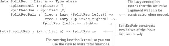
The Lazy type allows you to postpone a computation until the result is needed. For example, a variable of type Lazy Int is a computation that, when evaluated, will produce a value of type Int. Idris has the following two functions built-in:
Delay : a -> Lazy a Force : Lazy a -> a
When type-checking, Idris will insert applications of Delay and Force implicitly, as required. Therefore, in practice, you can treat Lazy as an annotation that states that a variable will only be evaluated when its result is required. You’ll see the definition of Lazy in more detail in chapter 11.
Listing 10.9. Starting point for a total implementation of mergeSort, using SplitRec (MergeSortView.idr)

You can implement mergeSort using the SplitRec view by taking the following steps:
- Define— Begin by adding a with block, to say you’d like to write the function by using the SplitRec view:
mergeSort : Ord a => List a -> List a mergeSort input with (splitRec input) mergeSort [] | SplitRecNil = ?mergeSort_rhs_1 mergeSort [x] | SplitRecOne = ?mergeSort_rhs_2 mergeSort (lefts ++ rights) | (SplitRecPair lrec rrec) = ?mergeSort_rhs_3
- Refine— The inputs [] and [x] are already sorted:
mergeSort : Ord a => List a -> List a mergeSort input with (splitRec input) mergeSort [] | SplitRecNil = [] mergeSort [x] | SplitRecOne = [x] mergeSort (lefts ++ rights) | (SplitRecPair lrec rrec) = ?mergeSort_rhs_3
- Refine— For the (lefts ++ rights) case, you can sort lefts and rights recursively, and then merge the results:
mergeSort : Ord a => List a -> List a mergeSort input with (splitRec input) mergeSort [] | SplitRecNil = [] mergeSort [x] | SplitRecOne = [x] mergeSort (lefts ++ rights) | (SplitRecPair lrec rrec) = merge (mergeSort lefts | lrec) (mergeSort rights | rrec)
The | says that, in the recursive calls, you want to bypass constructing the view, because you already have appropriate views for lefts and rights.
You can confirm that the new definition of mergeSort is total, and test it on some examples:
*MergeSortView> :total mergeSort Main.mergeSort is Total *MergeSortView> mergeSort [3,2,1] [1, 2, 3] : List Integer *MergeSortView> mergeSort [5,1,4,3,2,6,8,7,9] [1, 2, 3, 4, 5, 6, 7, 8, 9] : List Integer
Exercises
These exercises use views defined in the Idris library in the modules Data.List.Views, Data.Vect.Views, and Data.Nat.Views. For each view mentioned in the exercises, use :doc to find out about the view and its covering function.For each of these exercises, make sure Idris considers your solution to be total.
- Implement an equalSuffix function using the SnocList view defined in Data.List.Views. It should have the following type:
equalSuffix : Eq a => List a -> List a -> List a
Its behavior should be to return the maximum equal suffix of the two input lists. Here’s an example:*ex_10_2> equalSuffix [1,2,4,5] [1..5] [4, 5] : List Integer *ex_10_2> equalSuffix [1,2,4,5,6] [1..5] [] : List Integer *ex_10_2> equalSuffix [1,2,4,5,6] [1..6] [4, 5, 6] : List Integer
- Implement mergeSort for vectors, using the SplitRec view defined in Data.Vect.Views.
- Write a toBinary function that converts a Nat to a String containing a binary representation of the Nat. You should use the HalfRec view defined in Data.Nat.Views. If you have a correct implementation, you should see this:
*ex_10_2> toBinary 42 "101010" : String *ex_10_2> toBinary 94 "1011110" : String
Hint: It’s okay to return an empty string if the input is Z. - Write a palindrome function that returns whether a list is the same when traversed forwards and backwards, using the VList view defined in Data.List.Views. If you have a correct implementation, you should see the following:
*ex_10_2> palindrome (unpack "abccba") True : Bool *ex_10_2> palindrome (unpack "abcba") True : Bool *ex_10_2> palindrome (unpack "abcb") False : Bool
Hint: The VList view allows you to traverse a list in linear time, processing the first and last elements simultaneously and recursing on the middle of the list.
10.3. Data abstraction: hiding the structure of data using views
The views you’ve seen so far in this chapter allow you to inspect and traverse data structures in ways beyond the default pattern matching, focusing in particular on List. In a sense, views allow you to describe alternative interfaces for building pattern-matching definitions:- Using SnocList, you can see how a list is constructed using [] and by adding a single element with ++, rather than using [] and ::.
- Using SplitRec, you can see how a list is constructed as an empty list, a singleton list, or a concatenation of a pair of lists.
That is, you can find out how a value was constructed by looking at the view, rather than by looking directly at the constructors of that value. In fact, you often won’t need to know what the data constructors of a value are to be able to use a view of a value.
With this in mind, one use of views in practice is to hide the representation of data in a module, while still allowing interactive type-driven development of functions that use that data, by case splitting on a view of that data.
The origin of views
The idea of views was proposed by Philip Wadler for Haskell in 1987, in his paper “Views: a way for pattern matching to cohabit with data abstraction.” The example in this section is in the spirit of Wadler’s paper, which contains several other examples of using views in practice. Views as a programming idiom, using dependent types and a notation similar to the with notation in Idris, was later proposed by Conor McBride and James McKinna in their 2004 paper, “The view from the left.”
To conclude this chapter, we’ll look at this idea in action. We’ll revisit the data store example that we implemented in chapters 4 and 6, hide the representation of the data in an Idris module, and export only the following:
- Schema descriptions, explaining the form of data in the store
- A function for initializing a data store, empty
- A function for adding an entry to the store, addToStore
- A view for traversing the contents of the store, StoreView, along with its covering function, storeView
None of these require users of the module to know anything about the structure of the store itself or the structure of the data contained within it.
Before you implement a module and export the relevant definitions, though, we’ll need to discuss briefly how Idris supports data abstraction in modules.
10.3.1. Digression: modules in Idris
With the exception of a small example in chapter 2, the programs you’ve written in this book have been self-contained in a single main module. As you write larger applications,
however, you’ll need a way to organize code into smaller compilation units, and to control which definitions are exported from those units.The following listing shows a small Idris module that defines a Shape type and exports it, along with its data constructors and a function to calculate the area of a shape.
Listing 10.10. A module defining shapes and area calculations (Shape.idr)
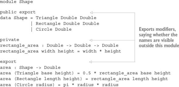
Each name defined in this module has an export modifier that explains whether that name is visible to other modules. An export modifier can be one of the following:
- private—The name is not exported at all.
- export—The name and type are exported, but not the definition. In the case of a data type, this means the type constructor is exported, but the data constructors are private.
- public export—The name, type, and complete definition are exported. For data types, this means the data constructors are exported. For functions, this means the functions’ definitions are exported.
If there’s no export modifier on a function or data type definition, Idris treats it as private. In the preceding example, this means that a module that imports Shape can use the names Shape, Triangle, Rectangle, Circle, and area, but not rectangle_area.
Exporting function definitions
Exporting a function’s definition as well as its type (via public export) is important if you want to use the function’s behavior in a type. In particular, this is important for type synonyms and type-level functions, which we first used in chapter 6.
The next listing shows an alternative version of the Shape module that keeps the details of the Shape data type abstract, exporting the type but not its constructors.
Listing 10.11. Exporting Shape as an abstract data type (Shape_abs.idr)
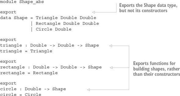
Using export modifiers, you can implement a module that implements the features of a data store but only exports functions for creating a store, adding items, and traversing the store, without exporting any details about the structure of the store.
10.3.2. The data store, revisited
To illustrate the role of views in data abstraction, we’ll create a module that implements a data store, exporting functions for constructing the store. We’ll also implement a view for inspecting and traversing the contents of the store.
The following listing shows the DataStore.idr module. This is a slight variation on the DataStore record you implemented in chapter 6.
Listing 10.12. Data store, with a schema (DataStore.idr)
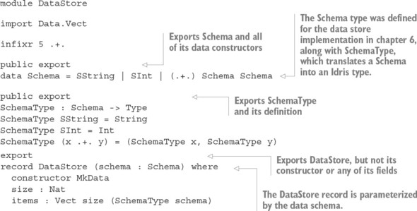
export record DataStore (schema : Schema) where constructor MkData size : Nat items : Vect size (SchemaType schema)
The syntax for a parameterized record declaration is similar to the syntax for an interface declaration, with the parameters and their types listed after the record name. This declaration gives rise to a DataStore type constructor with the following type:
DataStore : Schema -> Type
It also gives rise to functions for projecting the size of the store (size) and the entries in the store (items) out of the record. The functions have the following types:
size : DataStore schema -> Nat items : (rec : DataStore schema) -> Vect (size rec) (SchemaType schema)
Because the record has the export modifier export, the DataStore data type is visible to other modules, but the size and items projection functions aren’t.
Listing 10.13 shows three functions that other modules can use to create a new, empty store with a specific schema (empty), or add a new entry to a store (addToStore). Each of these functions has the export modifier export, meaning that other modules can see their names and types but have no access to their definitions.
Listing 10.13. Functions for accessing the store (DataStore.idr)
export empty : DataStore schema empty = MkData 0 [] export addToStore : (value : SchemaType schema) -> (store : DataStore schema) -> DataStore schema addToStore value (MkData _ items) = MkData _ (value :: items)
To be able to use this module effectively, you’ll also need to traverse the entries in the store. You can build the contents of a store using empty to create a new store and addToStore to add a new entry. It would therefore be convenient to be able to use
these as patterns to match the contents of a store. When you match on a store, you’ll need to deal with the following two cases:- An empty case that matches a store with no contents
- An addToStore value store case that matches a store where the first entry is given by value, and the remaining items in the store are given by store
To match these cases, you can write a view of DataStore.
10.3.3. Traversing the store’s contents with a view
Listing 10.14 shows a StoreView view and its covering function, storeView. They allow you to traverse the contents of a store by seeing how the store was constructed, either with empty or addToStore.
Listing 10.14. A view for traversing the entries in a store (DataStore.idr)
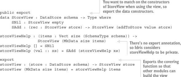
The StoreView view gives you access to the contents of the store by pattern matching but hides its internal representation. To use the store, and to traverse its contents, you don’t need to know anything about the internal representation.
To illustrate this, let’s set up some test data and write some functions to inspect it. The next listing defines a store and populates it with some test data, mapping planet names to the name of the space probe that first visited the planet and the year of the visit.[1]
We won’t, however, get into any debates about whether Pluto is a planet here.
1
Listing 10.15. A datastore populated with some test data (TestStore.idr)
import DataStore testStore : DataStore (SString .+. SString .+. SInt) testStore = addToStore ("Mercury", "Mariner 10", 1974) (addToStore ("Venus", "Venera", 1961) (addToStore ("Uranus", "Voyager 2", 1986) (addToStore ("Pluto", "New Horizons", 2015) empty))) When expressions get deeply nested, as in the testStore definition, it can be difficult to keep track of the bracketing. The $ operator is an infix operator that applies a function to an argument, and you can use it to reduce the need for bracketing.
Using it, you can write the following:
testStore = addToStore ("Mercury", "Mariner 10", 1974) $ addToStore ("Venus", "Venera", 1961) $ addToStore ("Uranus", "Voyager 2", 1986) $ addToStore ("Pluto", "New Horizons", 2015) $ empty Writing $ is therefore equivalent to putting the rest of the expression in brackets. For example, writing f x $ y z is exactly equivalent to writing f x (y z). The following listing shows a basic traversal of the data store, returning a list of entries in the store.
Listing 10.16. A function to convert the store’s contents to a list of entries (TestStore.idr)
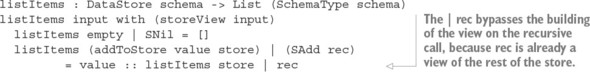
If you call showItems with the test data, you’ll see the following result:
*TestStore> listItems testStore [("Mercury", "Mariner 10", 1974), ("Venus", "Venera", 1961), ("Uranus", "Voyager 2", 1986), ("Pluto", "New Horizons", 2015)] : List (String, String, Int) More interestingly, you might want to write functions that traverse the data store and filter out certain entries. For example, suppose you want to get a list of the planets that were first visited by a space probe during the twentieth century. You could do this by writing the following function:
filterKeys : (test : SchemaType val_schema -> Bool) -> DataStore (SString .+. val_schema) -> List String
You can think of a schema of the form (SString .+. val_schema) as giving a key-value pair, where the key is a String and val_schema describes the form of the values.
Then, filterKeys will apply a function to the value in the pair, and if it returns True, it will add the key to a list of String. This can find the planets that a probe visited before the year 2000:*TestStore> filterKeys (\x => snd x < 2000) testStore ["Mercury", "Venus", "Uranus"] : List String
You can implement filterKeys using StoreView by taking the following steps:
- Type, define—Begin with a type and a skeleton definition:
filterKeys : (test : SchemaType val_schema -> Bool) -> DataStore (SString .+. val_schema) -> List String filterKeys test input = ?filterKeys_rhs
- Define— You’ll define the function by traversing the store using StoreView, so you can use the with construct to build the view, and case-split on it:
filterKeys : (test : SchemaType val_schema -> Bool) -> DataStore (SString .+. val_schema) -> List String filterKeys test input with (storeView input) filterKeys test empty | SNil = ?filterKeys_rhs_1 filterKeys test (addToStore value store) | (SAdd rec) = ?filterKeys_rhs_2
- Refine— If the store is empty, there’s no value to apply the test to, so return an empty list:
filterKeys : (test : SchemaType val_schema -> Bool) -> DataStore (SString .+. val_schema) -> List String filterKeys test input with (storeView input) filterKeys test empty | SNil = [] filterKeys test (addToStore value store) | (SAdd rec) = ?filterKeys_rhs_2
- Refine— Otherwise, because of the schema of the data store, entry must itself be a key-value pair:
filterKeys : (test : SchemaType val_schema -> Bool) -> DataStore (SString .+. val_schema) -> List String filterKeys test input with (storeView input) filterKeys test empty | SNil = [] filterKeys test (addToStore (key, value) store) | (SAdd rec) = ?filterKeys_rhs_2
You’ll apply test to the value. If the result is True, you’ll keep the key and recursively build the rest of the list. If the result is False, you’ll omit the key and build the rest of the list:filterKeys : (test : SchemaType val_schema -> Bool) -> DataStore (SString .+. val_schema) -> List String filterKeys test input with (storeView input) filterKeys test empty | SNil = [] filterKeys test (addToStore (key, value) store) | (SAdd rec) = if test value then key :: filterKeys test store | rec else filterKeys test store | rec
You can try this function with some test filters:*TestStore> filterKeys (\x => fst x == "Voyager 2") testStore ["Uranus"] : List String *TestStore> filterKeys (\x => snd x > 2000) testStore ["Pluto"] : List String *TestStore> filterKeys (\x => snd x < 2000) testStore ["Mercury", "Venus", "Uranus"] : List String
For both showItems and filterKeys, you’ve written a function that traverses the contents of the data store without knowing anything about the internal representation of the store. In each case, you’ve used a view to deconstruct the data, rather than deconstructing the data directly. If you were to change the internal representation in the DataStore module, and correspondingly the implementation of storeView, the implementations of showItems and filterKeys would remain unchanged.
Exercises
- Write a getValues function that returns a list of all values in a DataStore. It should have the following type:
getValues : DataStore (SString .+. val_schema) -> List (SchemaType val_schema)
You can test your definition by writing a function to set up a data store:testStore : DataStore (SString .+. SInt) testStore = addToStore ("First", 1) $ addToStore ("Second", 2) $ emptyIf you’ve implemented getValues correctly, you should see the following:*ex_10_3> getValues testStore [1, 2] : List Int
- Define a view that allows other modules to inspect the abstract Shape data type in listing 10.11. You should be able to use it to complete the following definition:
area : Shape -> Double area s with (shapeView s) area (triangle base height) | STriangle = ?area_rhs_1 area (rectangle width height) | SRectangle = ?area_rhs_2 area (circle radius) | SCircle = ?area_rhs_3
If you have implemented this correctly, you should see the following:*ex_10_3> area (triangle 3 4) 6.0 : Double *ex_10_3> area (circle 10) 314.1592653589793 : Double
10.4. Summary
- A view is a dependent type that describes the possible forms of another data type. Views take advantage of dependent pattern matching to allow you to extend the forms of patterns you can use.
- A covering function builds a view of a value. By convention, its name is the name of the view with an initial lowercase letter.
- The with construct allows you to use views directly, without defining an intermediate function.
- You can use views to define alternative traversals of data structures, such as extracting the last element of a list instead of the first.
- Recursive views help you write functions that are guaranteed to terminate, by writing recursive functions that pattern-match on the view.
- Idris provides several views for alternative traversals of List in the Data.List.Views library. Similar libraries exist for Vect, Nat, and String.
- You can hide the structure of data in a module, while still supporting interactive type-driven programming with that data, by exporting views for traversing data structures.
Part 3. Idris and the real world
In part 2, you gained experience in developing programs interactively, guided by types, and you learned about all of the core features of Idris. Now, it’s time to apply what you’ve learned to some more practical examples.
First, in chapter 11, you’ll learn about writing programs that deal with potentially infinite structures such as streams. You’ve learned about the importance of writing total functions, but in chapter 11 you’ll see that totality is about more than termination. A function is also total if it produces some portion of a potentially infinite result, which means you can write interactive systems such as servers and read-eval-print loops that run forever, but which are nevertheless total.
Chapters 12–14 deal with state. Real-world programs usually need to deal with global state somehow, and you’ll see both how to represent state and how to describe properties of state in such a way that you can guarantee that programs follow protocols accurately. If you’re implementing a system with important security properties, such as an ATM for a bank, you can use type-driven development to ensure that those properties are satisfied.
Finally, chapter 15 provides an extended example of type-driven development, showing how to implement a library for concurrent programming with types. You’ll start by writing a simple type to capture a specific concurrent programming problem, and then gradually refine it to capture more of the important properties of concurrent programs.
Chapter 11. Streams and processes: working with infinite data
This chapter covers
- Generating and processing streams of data
- Distinguishing terminating from productive total functions
- Defining total interactive processes using infinite streams
The functions we’ve written in this book so far have worked in batch mode, processing all of their inputs and then returning an output. In the previous chapter, we also spent some time discussing why termination is important, and you learned how to use views to help you write programs that are guaranteed to terminate.
But input data doesn’t always arrive in a batch, and you’ll often want to write programs that don’t terminate, running indefinitely. For example, it can be convenient to think of input data to an interactive program (such as keypresses, mouse movements, and so on) as a continuous stream of data, processed one element at a time, leading to a stream of output data. In reality, many programs are, in effect, stream processors:
- A read-eval-print loop, such as the Idris environment, processes a potentially infinite stream of user commands, giving an output stream of responses.
- A web server processes a potentially infinite stream of HTTP requests, giving an output stream of responses to be sent over the network.
- A real-time game processes a potentially infinite stream of commands from a controller, giving an output stream of audiovisual actions.
Furthermore, even when you’re writing pure functions that don’t interact with external data sources or devices, streams allow you to write reusable program components by separating the production of data from the consumption of data. For example, suppose you’re writing a function to determine the square root of a number. You can do this by producing an infinite list of successively closer approximations to a solution, and then writing a separate function to consume that list, finding the first approximation within the desired bounds.
Producing and consuming data
A common theme in this chapter is the distinction between programs that consume (or process) data, and programs that produce data. All the functions you’ve seen in this book so far have been consumers of data, and in the last chapter we looked at using views to help us write functions that are guaranteed to terminate when consuming data. When you’re writing terminating functions, however, consuming data is only part of the story: a function that generates an infinite stream is never going to terminate, after all. As you’ll see, Idris checks that functions that generate streams are guaranteed to be productive, so that any function that consumes the output of a stream generator will always have data to process.
The kinds of programs we write in practice often have a terminating component, processing and responding to user input, and a nonterminating component, which is an infinite loop that repeatedly invokes the terminating component. In this chapter, you’ll see how to write programs that manage this distinction, both producing and consuming potentially infinite data. We’ll start with one of the most common infinite structures, streams, and later look at how to define total functions describing interactive functions that execute indefinitely.
11.1. Streams: generating and processing infinite lists
Streams are infinite sequences of values, and you can process one value at a time. In this section, you’ll see how to write functions that produce an infinite sequence of data, as required, and how to write functions that consume finite portions of data produced as a stream.
As a first example, to illustrate the ideas behind streams, we’ll look at how to generate an infinite sequence of numbers, 0, 1, 2, 3, 4, ..., and how to process them as needed to label elements in a list, as illustrated in figure 11.1.
Figure 11.1. Labeling the elements of a List by taking elements from an infinite stream of numbers. The stream contains an infinite number of elements, but you only take as many as you need to label the elements in the finite list.
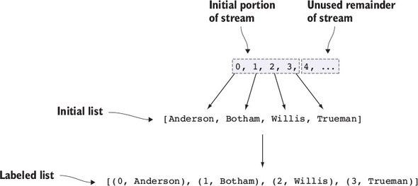
As well as showing you how to define potentially infinite data types, I’ll also introduce the Stream data type, provided by the Prelude, and we’ll briefly look at some functions on Streams. Finally, we’ll look at a larger example using a stream of random numbers to implement an arithmetic game.
11.1.1. Labeling elements in a List
Suppose you want to write a function that labels every element of a List with an integer indicating its position in the list, as in figure 11.1. That is, something like this:
label : List a -> List (Integer, a)
Running this function on some examples should give the following results:
*Streams> label ['a', 'b', 'c'] [(0, 'a'), (1, 'b'), (2, 'c')] : List (Integer, Char) *Streams> label ["Anderson", "Botham", "Willis", "Trueman"] [(0, "Anderson"), (1, "Botham"), (2, "Willis"), (3, "Trueman")] : List (Integer, String)
The following listing shows one way to write label by writing a helper function, labelFrom that takes the label for the first element of the list, and then labels the remainder of the list, incrementing the label.
Listing 11.1. Labeling each element of a list with an integer (Label.idr)
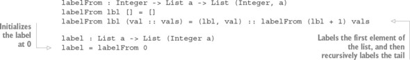
- countFrom—Generates an infinite stream of numbers, counting upwards from a given starting point.
- labelWith—Takes an infinite stream of labels, and pairs each label with a corresponding element in a finite list. It therefore only consumes as much of the infinite stream as necessary to label the elements in the list.
A natural way to try to write countFrom might be to generate a List of Integer from a given starting point:
countFrom : Integer -> List Integer countFrom n = n :: countFrom (n + 1)
When Idris runs a compiled program, however, it fully evaluates the arguments to a function before it evaluates the function itself. So, unfortunately, if you try to pass the result of countFrom to a function that expects a List, that function will never run because the result of countFrom will never be fully evaluated. If you ask Idris whether this definition of countFrom is total, it will tell you that there’s a problem:
*StreamFail> :total countFrom Main.countFrom is possibly not total due to recursive path: Main.countFrom, Main.countFrom
You can see that countFrom will never terminate, because it makes a recursive call for every input, but to write labelWith you’ll only need a finite portion of the result of countFrom. What you really need to know about countFrom, therefore, is not that it always terminates, but rather that it will always produce as many numbers as you need. That is, you need to know that it’s productive and is guaranteed to generate an indefinitely long sequence of numbers.
As you’ll see in the next section, you can use types to distinguish between those expressions for which evaluation is guaranteed to terminate and those expressions for which evaluation is guaranteed to keep producing new values, marking arguments to a data structure as potentially infinite.
11.1.2. Producing an infinite list of numbers
To generate an infinite list of numbers and consume only the finite portion of the list that you need, you can use a new data type, Inf, for marking the potentially infinite parts of the structure.You’ll see more details of how Inf works shortly. First, though, let’s take a look at a data type of infinite lists that uses Inf.
Listing 11.2. A data type of infinite lists (InfList.idr)
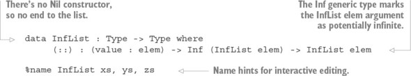
InfList is similar to the List generic type, with two significant differences:
- There’s no Nil constructor, only a (::) constructor, so there’s no way to end the list.
- The recursive argument is wrapped in a new data type, Inf, that marks the argument as potentially infinite.
To manipulate potentially infinite computations, you can use the Delay and Force functions. Listing 11.3 gives the types of Delay and Force. The idea is that you can use Delay and Force to control exactly when a subexpression is evaluated, so that you only calculate the finite portion of an infinite list that’s required for a specific function.
Listing 11.3. The Inf abstract data type, for delaying potentially infinite computations
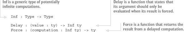
The following listing shows how you can define countFrom, generating an infinite list of Integers from a given starting value.
Listing 11.4. Defining countFrom as an infinite list (InfList.idr)
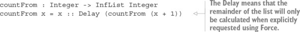
*InfList> countFrom 0 0 :: Delay (countFrom 1) : InfList Integer
You can see that the Idris evaluator has left the argument to Delay unevaluated. The evaluator treats Force and Delay specially: it will only evaluate an argument to Delay when explicitly requested to by a Force. As a result, despite there being a recursive call to countFrom on every input, evaluation at the REPL still terminates. Idris even agrees that it’s total:
*InfList> :total countFrom Main.countFrom is Total
Terminology: recursion and corecursion, data and codata
You may hear Idris programmers referring to functions such as countFrom as corecursive rather than recursive, and infinite lists as codata rather than data. The distinction between data and codata is that data is finite and is intended to be consumed, whereas codata is potentially infinite and is intended to be produced. Whereas recursion operates by taking data and breaking it down toward a base case, corecursion operates by starting at a base case and building up codata.
It may seem surprising that Idris considers countFrom to be total, given that it produces an infinite structure. Before we continue discussing how to work with infinite lists, therefore, it’s worth investigating in more detail what it means for a function to be total.
11.1.3. Digression: what does it mean for a function to be total?
If a function is total, it will never crash due to a missing case (that is, all well-typed inputs are covered), and it will always return a well-typed result within a finite time. The functions you’ve written in previous chapters have all taken finite data as inputs, so they’re total as long as they terminate for all inputs. But now that you’ve seen the Inf type, you’re able to write functions that produce infinite data, and these functions don’t terminate! We’ll therefore need to refine our understanding of what it means for a function to be total.
Functions that produce infinite data can be used as components of terminating functions, provided they’ll always produce a new piece of data on request. In the case of countFrom, it will always produce a new Integer before making a delayed recursive call.
Figure 11.2 illustrates the structure of countFrom. The delayed recursive call to countFrom is an argument to (::), meaning that countFrom will always produce at least one element of an infinite list before making a recursive call. Therefore, any function that consumes the result of countFrom will always have data to work with.
Figure 11.2. Producing values of an infinite structure. The Delay means that Idris will only make the recursive call to countFrom when it’s required by Force.
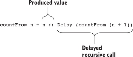
- Terminates with a well-typed result
- Produces a non-empty finite prefix of a well-typed infinite result in finite time
We can describe total functions as either terminating or productive. The halting problem is the difficulty of determining whether a specific program terminates or not, and, thanks to Alan Turing, we know that it’s impossible in general to write a program that solves the halting problem. In other words, Idris can’t determine whether one of these conditions holds for all total functions. Instead, it makes a conservative approximation by analyzing a function’s syntax.
Idris considers a function to be total if there are patterns that cover all well-typed inputs, and it can determine that one of the following conditions holds:
- When there’s a recursive call (or a sequence of mutually recursive calls), there’s a decreasing argument that converges toward a base case.
- When there’s a recursive call as an argument to Delay, the delayed call will always be an argument to a data constructor (or sequence of nested data constructors) after evaluation, for all inputs.
We discussed the first of these conditions in the previous chapter. The second condition allows us to use functions like countFrom in a terminating function. To illustrate this further, it’s helpful to see how the resulting infinite list is used. As an example, let’s write a function that consumes a finitely long prefix of an InfList.
11.1.4. Processing infinite lists
A function that generates an InfList is total provided that it’s guaranteed to keep producing data whenever data is required. You can see how this works by writing a program that calculates a finite list from the prefix of an infinite list:
getPrefix : (count : Nat) -> InfList ty -> List tygetPrefix returns a List consisting of the first count items from an infinite list. It works by recursively taking the next element from the infinite list as long as it needs more elements. You can define it with the following steps:
- Define— First, case-split on the count argument:
getPrefix : (count : Nat) -> InfList a -> List a getPrefix Z xs = ?getPrefix_rhs_1 getPrefix (S k) xs = ?getPrefix_rhs_2
- Refine— If you’re taking zero elements from the infinite list, return an empty list:
getPrefix : (count : Nat) -> InfList a -> List a getPrefix Z xs = [] getPrefix (S k) xs = ?getPrefix_rhs_2
- Define— If you’re taking more than one element, you’ll case-split on the infinite list and then add the first value in the infinite list as the first element of the result.
getPrefix : (count : Nat) -> InfList a -> List a getPrefix Z xs = [] getPrefix (S k) (value :: xs) = value :: ?getPrefix_rhs_1
- Type, refine—If you look at the type of the hole, ?getPrefix_rhs_1, you’ll see the following:
a : Type k : Nat value : a xs : Inf (InfList a) -------------------------------------- getPrefix_rhs_1 : List a
You can see from the type of xs that it’s an infinite list that has not yet been computed, because it’s an infinite list wrapped in an Inf. To complete the definition, you can Force the computation of xs and recursively get its prefix:getPrefix : (count : Nat) -> InfList a -> List a getPrefix Z xs = [] getPrefix (S k) (value :: xs) = value :: getPrefix k (Force xs)
The resulting definition is total, according to Idris:
*InfList> :total getPrefix Main.getPrefix is Total
Even though one of the inputs is potentially infinite, getPrefix will only evaluate as much as is necessary to retrieve count elements from the infinite list. Because count is a finite number, getPrefix will always terminate as long as the InfList is guaranteed to continue producing new elements.
In practice, you can omit calls to Delay and Force and let Idris insert them where required. If, during type checking, Idris encounters a value of type Inf ty when it
requires a value of type ty, it will add an implicit call to Force. Similarly, if it encounters a ty when it requires an Inf ty, it will add an implicit call to Delay. The following listing shows how you can define countFrom and getPrefix using implicit Force and Delay.Listing 11.5. Taking a finite portion of an infinite list, with implicit Force and Delay (InfList.idr)
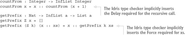
You can therefore treat Inf as an annotation on a type, mark the parts of a data structure that may be infinite, and let the Idris type checker manage the details of when computations must be delayed or forced.
Now that you’ve seen how to separate the production of data, using countFrom to generate an infinite list of numbers, from the consumption of data, using a function like getPrefix, we can revisit the definition of label. Rather than using our own InfList data type and countFrom, we’ll use a data type defined in the Prelude for this purpose: Stream.
11.1.5. The Stream data type
Listing 11.6 shows the definition of Stream in the Prelude. It has the same structure as the definition of InfList you saw in the previous section. Additionally, the Prelude provides several useful functions for building and manipulating Streams, some of which this listing also shows.
Listing 11.6. The Stream data type and some functions, defined in the Prelude
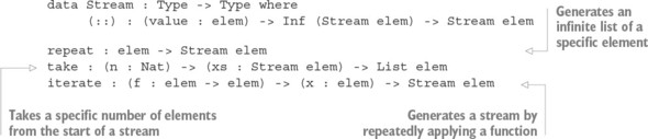
You can see the functions repeat, take, and iterate in action at the REPL. For example, repeat generates an infinite sequence of an element, delayed until specifically requested:
Idris> repeat 94 94 :: Delay (repeat 94) : Stream IntegerLike getPrefix on InfList, take takes a prefix of a Stream of a specific length:
Idris> take 10 (repeat 94) [94, 94, 94, 94, 94, 94, 94, 94, 94, 94] : List Integer
iterate applies a function repeatedly, generating a stream of the results. For example, starting at 0 and repeatedly applying (+1) leads to a sequence of increasing integers, like countFrom:
Idris> take 10 (iterate (+1) 0) [0, 1, 2, 3, 4, 5, 6, 7, 8, 9] : List Integer
Idris provides a concise syntax for generating streams of numbers, similar to the syntax for lists:
Idris> take 10 [1..] [1, 2, 3, 4, 5, 6, 7, 8, 9, 10] : List Integer
The syntax [1..] generates a Stream counting upwards from 1. This works for any countable numeric type, as in the following example:
Idris> the (List Int) take 10 [1..] [1, 2, 3, 4, 5, 6, 7, 8, 9, 10] : List Int
You can also change the increment:
Idris> the (List Int) (take 10 [1,3..]) [1, 3, 5, 7, 9, 11, 13, 15, 17, 19] : List Int
Putting all of this together, the following listing shows how to define label using iterate to generate an infinite sequence of integer labels, and a labelWith function that consumes enough of an infinite sequence of labels to attach a label to each element of a List.
Listing 11.7. Labeling each element of a List using a Stream (Streams.idr)
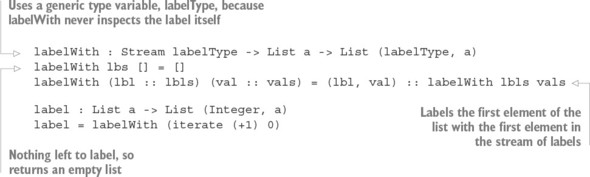
You can even give a more generic type to labelWith, taking a Stream labelType rather than a Stream Integer, and allow labeling by any type for which you can generate a Stream. For example, the cycle function generates a Stream that repeats a given sequence:
*Streams> take 10 $ cycle ["a", "b", "c"] ["a", "b", "c", "a", "b", "c", "a", "b", "c", "a"] : List String
Using cycle to generate a Stream, you could label each element of a List with a cycling sequence of labels, repeated as many times as necessary to label the entire list:
*Streams> labelWith (cycle ["a", "b", "c"]) [1..5] [("a", 1), ("b", 2), ("c", 3), ("a", 4), ("b", 5)] : List (String, Integer) 11.1.6. An arithmetic quiz using streams of random numbers
You can use a Stream in any situation where you need a source of data but don’t know in advance how much data you’ll need to generate. For example, you could write an interactive arithmetic quiz that takes a source of numbers for the questions. The following listing shows how you might do this.
Listing 11.8. An arithmetic quiz, taking a Stream of numbers for the questions (Arith.idr)
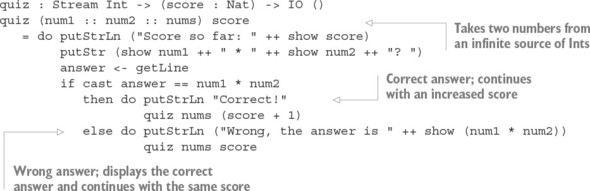
The quiz function takes an infinite source of Ints and the score so far, and then returns an IO action that displays the score and a question, reads an answer from the user, and repeats. The questions arise directly from the input stream, so you could try with a sequence of increasing numbers:
*Arith> :exec quiz (iterate (+1) 0) 0 Score so far: 0 0 * 1? 0 Correct! Score so far: 1 2 * 3? 6 Correct! Score so far: 2 4 * 5? 20 Correct! Score so far: 3
Aborting execution
Execution of a repeatedly looping program will continue until some external event causes the program to exit. You can abort execution at the REPL by pressing Ctrl-C.So far, this isn’t especially interesting because you know in advance what the questions will be. Instead, you could write a function that generates a stream of pseudo-random Ints generated from an initial seed. The following listing shows one way to generate a random-looking stream of numbers using a linear congruential generator.
Listing 11.9. Generating a stream of pseudo-random numbers from a seed (Arith.idr)
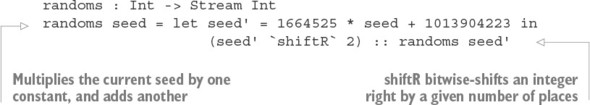
Pseudo-random number generation
The randoms function in listing 11.9 generates a random-looking, but predictable, stream of numbers from an initial seed, using a linear congruential generator. This is one of the oldest techniques for pseudo-random number generation. It suits our purposes for this example, but it’s not suitable for situations where high-quality randomness is required, such as cryptographic applications, due to the distribution and predictability of the generated numbers.
You could try running quiz with a stream of numbers generated by randoms:
*Arith> :exec quiz (randoms 12345) 0 Score so far: 0 1095649041 * -2129715532? no idea Wrong, the answer is -765659660 Score so far: 0
Earlier, the questions were too predictable, but now they’re perhaps a little too hard for most of us! Furthermore, in the preceding example, the result has even overflowed the bounds of an Int, so the reported answer is incorrect. Instead, the next listing shows one way to process the results of randoms so that they’re within reasonable bounds for an arithmetic quiz.
Listing 11.10. Generating suitable inputs for quiz (Arith.idr)
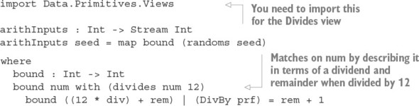
data Divides : Int -> (d : Int) -> Type where DivByZero : Int.Divides x 0 DivBy : (prf : rem >= 0 && rem < d = True) -> Int.Divides ((d * div) + rem) d divides : (val : Int) -> (d : Int) -> Divides val d
Note that in the DivBy case, you also have a proof that the remainder is guaranteed to have a value between 0 and the divisor by using the equality type = introduced in chapter 8.
You can use arithInputs as a source of random inputs for quiz and be sure that all the questions will use numbers between 1 and 12. Here’s an example:
*Arith> :exec quiz (arithInputs 12345) 0 Score so far: 0 2 * 1? 2 Correct! Score so far: 1 6 * 2? 18 Wrong, the answer is 12 Score so far: 1 11 * 10? 110 Correct! Score so far: 2
You’ve successfully used a source of random Ints as inputs to the quiz, and because randoms (and hence arithInputs) produces an infinite sequence of numbers, you’ll be able to generate new numbers as long as you need to.
There is, however, one remaining problem, which is that quiz itself is not total:
*Arith> :total quiz Main.quiz is possibly not total due to recursive path: Main.quiz, Main.quiz
This shouldn’t really surprise you, because there’s nothing in the definition of quiz that allows it to terminate. Instead, like countFrom, randoms, and arithInputs, it’s reading user input and continually producing an infinite sequence of IO actions.
In practice, interactive programs often have an outer loop, which you can run indefinitely, invoking specific commands, each of which you’d like to terminate so that you can issue the next command. The way to write interactive programs that run indefinitely, therefore, is to distinguish the types of interactive programs that describe terminating sequences of actions (commands in our main loop) from the types of interactive programs that describe possibly infinite sequences of actions (the main loop itself). We’ll explore this further in the next section.Exercises
- Write an every_other function that produces a new Stream from every second element of an input Stream. If you’ve implemented this correctly, you should see the following:
*ex_11_1> take 10 (every_other [1..]) [2, 4, 6, 8, 10, 12, 14, 16, 18, 20] : List Integer
- Write an implementation of Functor (as described in section 7.3.1) for InfList. If you’ve implemented this correctly, you should see the following, using countFrom and getPrefix as defined in section 11.1.4:
*ex_11_1> getPrefix 10 (map (*2) (countFrom 1)) [2, 4, 6, 8, 10, 12, 14, 16, 18, 20] : List Integer
- Define a Face data type that represents the faces of a coin: heads or tails. Then, define this:
coinFlips : (count : Nat) -> Stream Int -> List Face
This should return a sequence of count coin flips using the stream as a source of randomness. If you’ve implemented this correctly, you should see something like the following:*ex_11_1> coinFlips 6 (randoms 12345) [Tails, Heads, Tails, Tails, Heads, Tails] : List Face
Hint: It will help to define a function, getFace : Int -> Face. - You can define a function to calculate the square root of a Double as follows:
- Generate a sequence of closer approximations to the square root.
- Take the first approximation that, when squared, is within a desired bound from the original number.
square_root_approx : (number : Double) -> (approx : Double) -> Stream Double
Here, you’re looking for the square root of number, starting from an approximation, approx. You can generate the next approximation using this formula:next = (approx + (number / approx)) / 2
If you’ve implemented this correctly, you should see the following:*ex_11_1> take 3 (square_root_approx 10 10) [10.0, 5.5, 3.659090909090909] : List Double *ex_11_1> take 3 (square_root_approx 100 25) [25.0, 14.5, 10.698275862068964] : List Double
- Write a function that finds the first approximation of a square root that’s within a desired bound, or within a maximum number of iterations:
square_root_bound : (max : Nat) -> (number : Double) -> (bound : Double) -> (approxs : Stream Double) -> Double
This should return the first element of approxs if max is zero. Otherwise, it should return the first element (let’s call it val) for which the difference between val x val and number is smaller than bound. If you’ve implemented this correctly, you should be able to define square_root as follows, and it should be total:square_root : (number : Double) -> Double square_root number = square_root_bound 100 number 0.00000000001 (square_root_approx number number)
You can test it with the following values:*ex_11_1> square_root 6 2.449489742783178 : Double *ex_11_1> square_root 2500 50.0 : Double *ex_11_1> square_root 2501 50.009999000199954 : Double
11.2. Infinite processes: writing interactive total programs
When you write a function to generate a Stream, you give a prefix of the Stream and generate the remainder recursively. This is similar to quiz in that you give the initial IO actions to run and then generate the remainder of the IO actions recursively. So, you can think of an interactive program as being a program that produces a potentially infinite sequence of interactive actions.
In chapter 5, you wrote interactive programs using the IO generic type, where IO ty is the type of terminating interactive actions giving a result of type ty. In this section, you’ll see how to write nonterminating, but productive (and therefore total), interactive programs by defining an InfIO type for representing infinite sequences of IO actions.
Because InfIO describes infinite sequences of actions, the functions must be productive, so you can be certain that the resulting programs continue to produce new IO actions for execution while continuing to run forever. But InfIO merely describes sequences of interactive actions, so you’ll also need to write a function to execute those actions.
Overall, we’ll take the following approach to writing interactive total programs:- Define a type InfIO that describes infinite sequences of interactive actions.
- Write nonterminating but productive functions using InfIO.
- Define a run function that converts InfIO programs to IO actions.
Your first implementation of run will not, itself, be total. You’ll then see how to refine the definition so that even run is total, using a data type to describe how long execution should continue. First, though, you’ll need to see how to describe infinite processes by defining InfIO.
11.2.1. Describing infinite processes
The following listing shows how to define the InfIO type. It’s similar to Stream, except that, in an interactive program, you may want the value produced by the first action to influence the rest of a computation.
Listing 11.11. Infinite interactive processes (InfIO.idr)
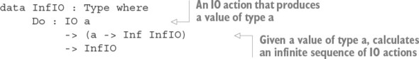
There are two arguments to Do:
- A description of an IO action to execute
- The remainder of the infinite sequence of actions. Because its type is a -> Inf InfIO, it can use the result produced by the first action to compute the remaining actions.
By using Inf to mark the remainder of the sequence as infinite, you’re telling Idris that you expect functions that return a value of type InfIO to be productive. In other words, as with functions on Stream, delayed recursive calls that produce an InfIO must be arguments to a constructor. The following listing shows how this works in a recursive program that repeatedly displays a message.
Listing 11.12. An infinite process that repeatedly displays a message (InfIO.idr)

The recursive call to loopPrint is an argument to the constructor Do, and loopPrint is guaranteed to produce a constructor (Do) as a finite prefix of its result. This satisfies the definition of a productive total function from section 11.1.3, so Idris is happy that loopPrint is total:
*InfIO> :total loopPrint Main.loopPrint is TotalRecall from chapter 5 that IO is a generic type describing interactive actions and that it will be executed by the runtime system. If you try evaluating loopPrint at the REPL, you’ll see a description of the first IO action that will be executed and the delayed remainder of the infinite sequence of actions:
*InfIO> loopPrint "Hello" Do (io_bind (prim_write "Hello!\n") (\__bindx => io_return ())) (\underscore => Delay (loopPrint "Hello")) : InfIO
Just as with IO, for this to be useful in practice, you’ll also need to be able to execute infinite sequences of actions.
11.2.2. Executing infinite processes
In chapter 5, you learned how the Idris runtime system will execute programs of type IO ty, where ty is the type of value produced by an interactive computation. So, in order to execute a value of type InfIO, you’ll need to start by converting it to an IO (). Here’s one way to do this.
Listing 11.13. Converting an expression of type InfIO to an executable IO action (InfIO.idr)
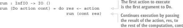
Using run, you can convert your function that repeatedly prints a message to an IO action, and execute it using :exec:
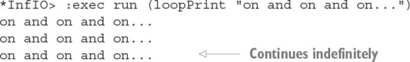
Because this runs indefinitely, at least until you abort it by pressing Ctrl-C, you should perhaps not be surprised to find that Idris doesn’t consider run to be total:
*InfIO> :total run Main.run is possibly not total due to recursive path: Main.run, Main.run
You know that loopPrint will continue to produce new IO actions to execute, because it’s total. This is valuable because a program that continues to execute IO actions is going to continue to make visible progress (at least assuming those actions produce some output, which we’ll consider further in section 11.3.2). It would be nice if run were also total, so that you’d at least know that all possible IO actions are processed and
that there isn’t any unexpected nontermination caused by the implementation of run itself.This would seem to be impossible: the only way to have a total, nonterminating function is to use the Inf type, and IO is a type of terminating action that doesn’t use Inf. And, indeed, if you want functions to execute indefinitely at runtime, you’ll need at least some way to escape from total functions. You can, however, try to make the escape as quietly as possible.
To achieve this, we’ll begin by making a terminating version of run that takes as an argument an upper bound on the number of actions it’s willing to execute.
11.2.3. Executing infinite processes as total functions
Earlier, in section 11.1.4, you wrote a getPrefix function that retrieved a finite portion of an infinite list:
getPrefix : (count : Nat) -> InfList a -> List a
You can think of the count argument as being the “fuel” that allows you to continue processing the infinite list. Once you run out of fuel, you can’t process any more of the list. You can do something similar for run, giving it an additional argument standing for the number of iterations it will run.
The following listing defines a Fuel data type and gives a new, total, definition of run that will execute actions as long as fuel remains.
Listing 11.14. Converting an expression of type InfIO to an executable IO action running for a finite time (InfIO.idr)
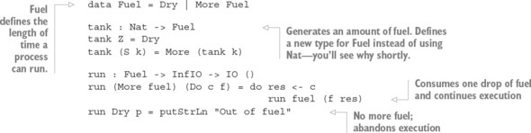
Now, run is total:
*InfIO> :total run Main.run is Total
Unfortunately, you still have a problem because you now need to specify an explicit maximum number of actions a program is allowed to execute, so you don’t really have indefinitely running processes anymore! For example:
*InfIO> :exec run (tank 5) (loopPrint "vroom") vroom vroom vroom vroom vroom Out of fuelIt’s valuable to ensure that run is total, because it guarantees that the implementation of run itself won’t be the cause of any unexpected nontermination. If you still want programs to run indefinitely, though, you’ll need to find a way to generate fuel indefinitely. You can achieve this by using the Lazy data type.
11.2.4. Generating infinite structures using Lazy types
If you have a means of generating infinite Fuel, you can run interactive programs indefinitely. Listing 11.15 shows how you can do this using a single nontotal function, forever. You also need to change the definition of Fuel so that it’s explicit in the type that you only generate Fuel when it’s required.
Listing 11.15. Generating infinite fuel (InfIO.idr)
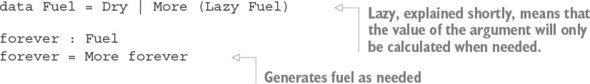
forever and nontermination
It’s necessary for forever to be nontotal because it (deliberately) introduces nontermination. Fortunately, this is the only nontotal function you need in order to be able to execute programs forever.
The purpose of Lazy is to control when Idris evaluates an expression. As the name Lazy implies, Idris won’t evaluate an expression of type Lazy ty until it’s explicitly requested by Force, which returns a value of type ty. The Prelude defines Lazy similarly to Inf, which you defined in section 11.1.2:
Lazy : Type -> Type Delay : (value : ty) -> Lazy ty Force : (computation : Lazy ty) -> ty
Also, like Inf, Idris inserts calls to Delay and Force implicitly. In fact, Inf and Lazy are sufficiently similar that they’re implemented internally using the same underlying type, as the next listing shows. The only difference in practice between Inf and Lazy is the way the totality checker treats them, as explained in the sidebar.
Listing 11.16. Internal definition of Inf and Lazy
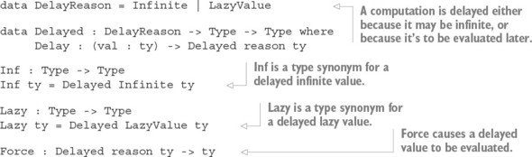
- If the argument has type Lazy ty, for some type ty, it’s considered smaller than the constructor expression.
- If the argument has type Inf ty, for some type ty, it’s not considered smaller than the constructor expression, because it may continue expanding indefinitely. Instead, Idris will check that the overall expression is productive, as discussed in section 11.1.3.
If you used Inf for Fuel, rather than Lazy, run would no longer be total because the argument, fuel, wouldn’t be considered smaller than the expression More fuel.
You’ve implemented three functions: loopPrint, which is the interactive program; run, which executes interactive programs given fuel; and forever, which provides an indefinite quantity of fuel. To summarize:
- loopPrint is a total function because it continues to produce IO actions indefinitely.
- run is a total function because it will consume IO actions, executing them as long as there is Fuel available.
- forever is a nontotal (or partial) function because it will never terminate and doesn’t produce any data inside an Inf type.
By writing a version of run that will process data as long as fuel is available, Idris can guarantee that run is total, consuming fuel as it goes. You still have an “escape hatch” that allows you to run interactive programs indefinitely, in the form of the forever function. Nevertheless, forever is the only function that’s not total.
You can still improve the definition of loopPrint itself. When we wrote interactive programs in chapter 5, we used do notation to help make interactive programs more readable, but we haven’t been able to do so using InfIO. You can, however, extend do notation to support your own data types, like InfIO.
11.2.5. Extending do notation for InfIO
As you saw in chapter 5, do notation translates to applications of the (>>=) operator, as illustrated again in figure 11.3.Figure 11.3. Transforming do notation to an expression using the >>= operator when sequencing actions

You’ve seen this transformation for IO in chapter 5, for Maybe in chapter 6, and in general for implementations of the Monad interface in chapter 7. In fact, the transformation is purely syntactic, so you can define your own implementations of (>>=) to use do notation for your own types. The following listing shows how you can define do notation for InfIO.
Listing 11.17. Defining do notation for infinite sequences of actions
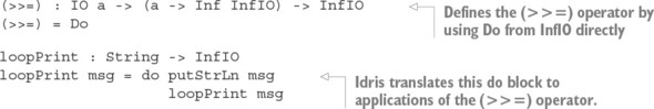
Idris translates the do block to applications of (>>=) and decides which version of (>>=) to use by looking at the required type. Here, because the required type of the overall expression is InfIO, it uses the version of (>>=) that produces a value of type InfIO.
The InfIO type allows you to describe infinitely running interactive programs, and by defining a (>>=) operator, you can write those programs in much the same way as programs with IO, provided that the final action is to call a function of type InfIO.
Now that you've seen that you can write productive interactive programs using do notation, we can revisit the arithmetic quiz from section 11.1.6.
11.2.6. A total arithmetic quiz
To conclude this section, we’ll update the arithmetic quiz so that it’s a total function, and you’ll see how you can incorporate this in a complete Idris program. Listing 11.18 shows our starting point, setting up the InfIO type and run function, as you’ve seen earlier in this section. You’ll need Data.Primitives.Views for generating the stream of random numbers. You’ll also import the System module for the time function, which you’ll use to help initialize the stream of random numbers.
Listing 11.18. Setting up InfIO (ArithTotal.idr)
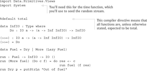
Idris supports a number of compiler directives that change certain details about the language. In listing 11.18, the %default total directive means that Idris will report an error if there are any functions that it can’t guarantee to be total.
You can override this for individual functions with the partial keyword. For example, forever is not total:
partial forever : Fuel forever = More forever
It’s a good idea to use %default total in your programs, because if Idris can’t determine that a function is either terminating or productive, this can be a sign that there’s a problem with the function’s definition. Furthermore, explicitly marking which functions are partial means that if there’s a problem with nontermination, or a program that crashes due to missing input, you’ve minimized the number of functions that could cause the problem.
Listing 11.19. Defining a total quiz function (ArithTotal.idr)
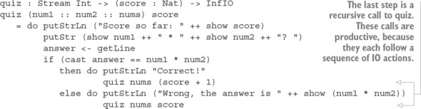
The final step is to write a main function that calls run to execute quiz with a stream of Ints. Here are the remaining parts of the implementation.
Listing 11.20. Completing the implementation with main (ArithTotal.idr)
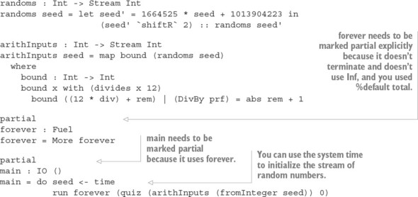
You’ve used randoms and arithInputs, as defined in section 11.1.6, to generate the stream of Ints. By using the system time to initialize the stream, you’ll get different questions every time you run the program.
In the whole implementation, the only functions that aren’t total are forever and main, the latter only because it needs to use forever to generate an indefinite amount of fuel for run. Because you used the %default total annotation, you needed to mark these as partial explicitly. That means you can be sure that the only possible cause of nontermination in the program is the fact that you’ve deliberately said that the program should run forever.
Other than forever, you know that the individual components will be one of the following:
- Productive— Such as quiz continuing to produce IO actions for interpretation and randoms continuing to produce new random numbers when required
- Terminating— Such as the individual IO commands and the generation of the next random number from a seed
This distinction is useful for writing realistic programs such as servers and REPLs, which you want to run indefinitely while being sure that each individual action the program executes terminates. Often, though, you’ll want more flexibility. At the moment, for example, you have no way to quit the quiz cleanly. We’ll return to this in the next section.
Exercise
The repl function defined in the Prelude isn’t total because it’s an IO action that loops indefinitely. Implement a new version of repl using InfIO:totalREPL : (prompt : String) -> (action : String -> String) -> InfIO
If you’ve implemented this correctly, totalREPL should be total, and you should be able to test it as follows:
*ex_11_2> :total totalREPL Main.totalREPL is Total *ex_11_2> :exec run forever (totalREPL "\n: " toUpper) : Hello [user input] HELLO : World [user input] WORLD
11.3. Interactive programs with termination
Using Inf, you can explicitly control when you want data to be produced, or when you want it to be consumed. As a result, you have a choice between programs that always terminate and programs that continue running forever. To write complete applications, though, you’ll need more control. After all, although you want a server to run indefinitely, you’d like to be able to shut it down cleanly when you want to.
So far, the types you’ve defined using Inf have had only one constructor, so they’ve required you to produce infinite sequences. Instead, you can mix infinite and finite components in a single data type, which means you can describe processes that can run indefinitely, but which are also allowed to terminate. In this section, you’ll see how to refine the InfIO type to support processes that terminate cleanly. Moreover, you’ll see how to introduce more precision into the type, and define a type of processes specifically for console I/O.
11.3.1. Refining InfIO: introducing termination
Using InfIO, you can write total interactive programs that are guaranteed to keep producing IO actions, running indefinitely. The following listing shows a small example of the form you saw in the previous section. This program repeatedly asks for the user’s name and displays a greeting.
Listing 11.21. Repeatedly greeting a user, running forever (Greet.idr)
greet : InfIO greet = do putStr "Enter your name: " name <- getLine putStrLn ("Hello " ++ name) greet Typically, when you write interactive programs, you’ll want to provide a means for the user to quit. Unfortunately, the only way a user can quit greet is by pressing Ctrl-C. There’s no way to write a function in InfIO that quits any other way! Fortunately, you can solve this with a small variation on InfIO. The Inf type marks a value as potentially infinite, rather than guaranteeing that the value is infinite, and you can introduce extra data constructors for potentially infinite types. You can define a new RunIO type, shown in the next listing, that adds a Quit constructor to describe programs that exit, producing a value.
Listing 11.22. The RunIO type, describing potentially infinite processes with an additional Quit command (RunIO.idr)
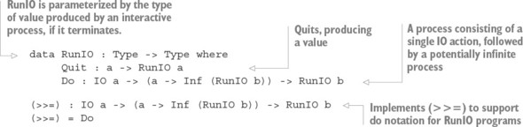
Using RunIO, you can write a version of greet, shown in the following listing, that quits when the user gives an empty input.
Listing 11.23. Repeatedly greets a user, exiting on empty input (RunIO.idr)
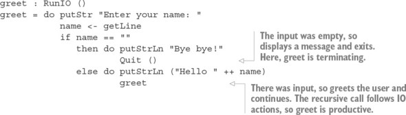
Depending on the input, greet is either terminating or productive. The totality checker accepts greet as total, because it satisfies the definition from section 11.1.3 that a total function either terminates or is productive for all well-typed inputs.
Before you can execute greet, you’ll need to write a new version of run that translates a program in RunIO to a sequence of IO actions for the runtime system to execute. Previously, run would only terminate on running out of Fuel, but now there are two possible reasons for termination:
- Running out of Fuel, as before
- Exiting cleanly, with a result, if the process being executed invokes Quit
The generic type Inf that you use in the type of potentially infinite structures follows a similar idea used in the Agda programming language, described by Nils Anders Danielsson in his 2010 paper “Total Parser Combinators.”
You can distinguish these results in the type:
run : Fuel -> RunIO a -> IO (Maybe a)
The possible results of run correspond to the two possible reasons for termination:
- If run runs out of Fuel, it returns Nothing.
- If run executes an action of the form Quit value, it returns Just value.
The following listing gives the new definition of run for RunIO.
Listing 11.24. Converting an expression of type RunIO ty to an executable action of type IO ty (RunIO.idr)
Finally, you can write a main program that executes greet and discards the result:
partial main : IO () main = do run forever greet pure ()
Because run now creates an IO action that produces a value of type Maybe () when invoked with greet, and main is expected to create an action that produces a value of type (), you need to finish by calling pure (). When you execute main at the REPL, you can now exit cleanly by entering an empty string:
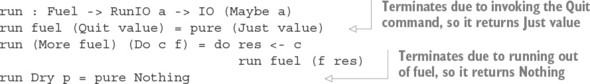
With RunIO, you’ve refined InfIO with the ability to terminate a process cleanly when required. This gives you more freedom to write interactive programs, but there’s
another way in which RunIO arguably gives you too much freedom. Specifically, a process described by RunIO is a sequence of arbitrary IO actions, giving you several possibilities, including these:- Reading from and writing to the console
- Opening and closing files
- Opening network connections
- Deleting files
For the programs you’ve written in this chapter, you’re only interested in the first of these. The others are not only unnecessary, but lead to the possibility of remote security vulnerabilities in the third case, and potentially destructive errors in the fourth.
One of the principles of type-driven development, which we discussed in chapter 1, is that we should aim to write types that describe as precisely as possible the values that inhabit that type. To conclude this chapter, therefore, we’ll look at how we can refine the RunIO type to describe only the actions that are necessary to implement the arithmetic quiz.
11.3.2. Domain-specific commands
You only need two IO actions when implementing the arithmetic quiz: reading from and writing to the console. Instead of allowing interactive programs in RunIO to execute arbitrary actions, therefore, you can restrict them to only the actions you need. That is, you can prevent your program from executing any interactive action that’s outside the problem domain in which you’re working.
The next listing shows a refined ConsoleIO type that describes interactive programs that support only reading from and writing to the console.
Listing 11.25. Interactive programs supporting only console I/O (ArithCmd.idr)
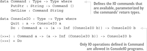
Effectively, Command defines an interactive interface that ConsoleIO programs can use. You can think of it as defining the capabilities or permissions of interactive programs, eliminating any unnecessary actions.
You now need to refine the implementation of run to be able to execute ConsoleIO programs.
Listing 11.26. Executing a ConsoleIO program (ArithCmd.idr)
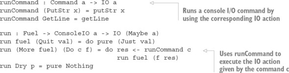
Domain-specific languages
A domain-specific language (DSL) is a language that’s specialized for a particular class of problems. DSLs typically aim to provide only the operations that are needed when working in a specific problem domain in a notation that’s accessible to experts in that domain, while eliminating any redundant operations.In a sense, ConsoleIO defines a DSL for writing interactive console programs, in that it restricts the programmer to only the interactive actions that are needed and eliminates unnecessary actions such as file processing or network communication.
Listing 11.27 shows how you can modify quiz to run as a ConsoleIO program. By looking at the type of quiz and the definitions of ConsoleIO and run, you have a guarantee that quiz will only execute console I/O actions. There’s no way it can open or close files, communicate over a network, or perform any other kind of interactive operation.
Listing 11.27. The arithmetic quiz, written as a ConsoleIO program (ArithCmd.idr)
To complete the implementation, you’ll need to implement a main function. The following listing shows a new implementation of main that executes the quiz and then displays the player’s final score after they enter quit.
Listing 11.28. A main function that executes the quiz and displays the final score (ArithCmd.idr)
Listing 11.29. Lifting out components of quiz into separate functions (ArithCmd.idr)
After quiz type-checks successfully, you can make several guarantees about its behavior by looking at the types and checking for totality:
- It will execute no interactive action other then putStr and getLine.
- It will either exit immediately or execute at least one interactive action, because it is productive.
- Every action executed will return a result in finite time, because it is total.
11.3.3. Sequencing Commands with do notation
In implementing quiz, you used two types to construct the function: Command and ConsoleIO:- Command describes single commands, which terminate.
- ConsoleIO describes sequences of terminating commands, which might be infinite.
So, you can have single, finite commands, or sequences of infinite commands. But it would also be useful to be able to construct composite commands; that is, sequences of commands that are guaranteed to terminate. For example, you might like to write a composite command that displays a prompt, and then reads and parses user input. The next listing shows a type that represents possible user inputs, and a skeleton definition of a function to read and parse input.
Listing 11.30. Defining a type for representing user input, and a composite command for reading and parsing input (ArithCmdDo.idr)
To write this function, you need to do the following:
- Display the prompt.
- Read an input from the console.
- Convert the input string to Input and return it.
Because Command currently supports only single commands, you’ll need to extend it to support sequences of commands. The next listing shows the extended definition, including two new data constructors, Pure and Bind, and a correspondingly updated definition of runCommand.
Listing 11.31. Extending Command to allow sequences of commands (ArithCmdDo.idr)
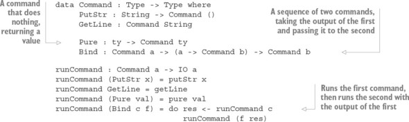
(>>=) : Command a -> (a -> Command b) -> Command b (>>=) = Bind
If you try this, Idris will complain that (>>=) is already defined, because you’ve defined do notation for ConsoleIO:
ArithCmdDo.idr:22:7:Main.>>= already defined
Idris allows multiple definitions of the same function name, as long as they’re in separate namespaces. You’ve already seen this with List and Vect, for example, where each has constructors called Nil and (::) that Idris disambiguates according to the context in which you use them.
The namespace is given by the module where you define functions. Namespaces are also hierarchical, so you can introduce further namespaces inside a module. You can have multiple definitions of functions called (>>=) in one module by introducing new namespaces for each. The following listing shows how you can define new namespaces for each (>>=).
Listing 11.32. Creating two definitions of (>>=) in separate namespaces (ArithCmdDo.idr)
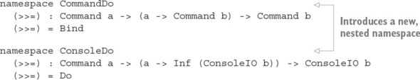
If you check the type of (>>=) at the REPL, you’ll see all the definitions of (>>=) in their respective namespaces, with their types:
*ArithCmdDo> :t (>>=) Main.CommandDo.(>>=) : Command a -> (a -> Command b) -> Command b Main.ConsoleDo.(>>=) : Command a -> (a -> Inf (ConsoleIO b)) -> ConsoleIO b Prelude.Monad.(>>=) : Monad m => m a -> (a -> m b) -> m b
You could also define an implementation of the Monad interface for Command, as described in chapter 7. When possible, this is often preferable because the Prelude and base libraries define several functions that work generically with Monad implementations. To do this, you’d also need to define implementations of Functor and Applicative. You’ll see an example of how to do this for a similar type in the next chapter.
You can’t, however, define an implementation of Monad for ConsoleIO, because the type of ConsoleDo.(>>=) doesn’t fit the type of the (>>=) method in the Monad interface.Using CommandDo.(>>=) to provide do notation, you can complete the definition of readInput.
Listing 11.33. Implementing readInput by sequence Command (ArithCmdDo.idr)
readInput : (prompt : String) -> Command Input readInput prompt = do PutStr prompt answer <- GetLine if toLower answer == "quit" then Pure QuitCmd else Pure (Answer (cast answer))
Finally, you can use readInput in the main quiz function to encapsulate the details of displaying a prompt and parsing the user’s input, shown in the final definition.
Listing 11.34. Defining quiz using readInput as a composite command to display a prompt and read user input (ArithCmdDo.idr)
In this final definition, you distinguish between terminating sequences of commands (using Command), and potentially nonterminating console I/O programs (using ConsoleIO). Syntactically, you write functions the same way in each, but the type tells you whether the function is allowed to run indefinitely, or whether it must eventually terminate.
Exercises
- Update quiz so that it keeps track of the total number of questions and then returns the number of correct answers and the number of questions attempted. A sample run might look something like this:
*ex_11_3> :exec Score so far: 0 / 0 9 * 11? 99 Correct! Score so far: 1 / 1 6 * 9? 42 Wrong, the answer is 54 Score so far: 1 / 2 10 * 2? 20 Correct! Score so far: 2 / 3 7 * 2? quit Final score: 2 / 3
- Extend the Command type from section 11.3.2 so that it also supports reading and writing files. Hint: Look at the types of readFile and writeFile in the Prelude to decide what types your data constructors should have.
- Use your extended Command type to implement an interactive “shell” that supports the following commands:
- cat [filename], which reads a file and displays its contents
- copy [source] [destination], which reads a source file and writes its contents to a destination file
- exit, which exits the shell
11.4. Summary
- You can generate infinite data using Inf to state which parts of a structure are potentially infinite.
- A total function either terminates with a well-typed input or produces a prefix of a well-typed infinite result in finite time.
- You can process infinite structures by using finite data to determine how much of the infinite structure to use.
- The Prelude defines a Stream data type for constructing infinite lists.
- You can define processes as infinite sequences of IO actions.
- To execute an infinite process, you define a function that takes an argument stating how long the process should run.
- The partial function forever allows processes to run indefinitely by generating an infinite amount of Fuel, using the Lazy type.
- By implementing (>>=), you can extend do notation for your own data types to make programs easier to read and write.
- You can mix finite and infinite structures within the same data type to define potentially infinite processes that may also terminate.
Chapter 12. Writing programs with state
This chapter covers
- Using the State type to describe mutable state
- Implementing custom types for state management
- Defining and using records for global system state
Idris is a pure language, so variables are immutable. Once a variable is defined with a value, nothing can update it. This might suggest that writing programs that manipulate state is difficult, or even impossible, or that Idris programmers in general aren’t interested in state. In practice, the opposite is true.
In type-driven development, a function’s type tells you exactly what a function can do in terms of its allowed inputs and outputs. So, if you want to write a function that manipulates state, you can do that, but you need to be explicit about it in the function’s type. In fact, we’ve already done this in earlier chapters:
- In chapter 4, we implemented an interactive data store using global state.
- In chapter 9, we implemented a word-guessing game using global state to hold the target word, the letters guessed, and the number of guesses still available.
- In chapter 11, we implemented an arithmetic game using global state to hold the user’s current score.
Almost all real-world applications need to manipulate state to some extent. Sometimes, as in the previous examples, state is global and is used throughout an application. Sometimes, state is local to an algorithm; for example, a graph-traversal algorithm will hold the nodes it has visited in local state to avoid visiting nodes more than once. In this chapter, we’ll look at how we can manage mutable state in Idris, both for state that’s local to an algorithm, and for representing overall system state.
State management and dependent types
We won’t use many dependent types in this chapter; using dependent types in state introduces some complications, as well as opportunities for precision in describing state transition systems and protocols. We’ll consider these opportunities in the next two chapters, but we’ll begin here by looking at how state works in general.
Previously, we’ve used types to describe interactive programs in terms of sequences of commands, using IO in chapter 5 and ConsoleIO in chapter 11. Stateful programs can work in the same way, using types to describe the operations a stateful program can perform. We’ll begin by looking at the generic State type defined in the Idris library and then at how we can define types like State ourselves. Finally, we’ll look at how we can structure a complete application with state, refining the arithmetic quiz from chapter 11.
12.1. Working with mutable state
Even though Idris is a pure language, it’s often useful to work with state. It’s particularly useful, when writing functions with a complex data structure, such as a tree or a graph, to be able to read and write local state as you’re traversing the structure. In this section, you’ll see how to manage mutable state.
Comparing state in Idris and Haskell
This section describes the State type for capturing local mutable state in Idris. If you’re familiar with Haskell, you’ll find that you can use State in Idris in the same way as Haskell, by importing Control.Monad.State. If you’re familiar with the State type in Haskell, you can safely move ahead to section 12.2, where I’ll describe a custom implementation of State.
In the previous chapter, you wrote a function to attach labels to elements of a list, taking the labels from a Stream. It’s repeated for reference here.
Listing 12.1. Labeling each element of a List using a Stream (Streams.idr)
12.1.1. The tree-traversal example
Figure 12.1 shows the result of a function that labels a binary tree, and we’ll use this as a running example throughout this section. This function labels the nodes depth first, left to right, so the deepest, leftmost node takes the first label, and the deepest, rightmost node takes the last label.
Figure 12.1. Labeling a tree, depth first. Each node is labeled with an integer.
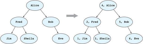
The following listing gives the definition of binary trees that we’ll use for labeling, along with testTree, a representation of the specific tree we’ll label (from the example in figure 12.1).
Listing 12.2. Definition of binary trees, and an example (TreeLabel.idr)
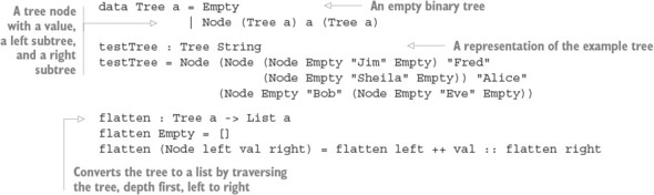
It’s convenient to define flatten so that you can easily see the ordering in which the labels should be applied:
*TreeLabel> flatten testTree ["Jim", "Fred", "Sheila", "Alice", "Bob", "Eve"] : List StringOnce you’ve written a treeLabel function that labels the nodes in the tree according to the elements in a stream, you should be able to run it as follows:
*TreeLabel> flatten (treeLabel testTree) [(1, "Jim"), (2, "Fred"), (3, "Sheila"), (4, "Alice"), (5, "Bob"), (6, "Eve")] : List (Integer, String)
When you wrote the function to label lists, in listing 12.1, you had a direct correspondence between the structure of the stream of labels and the list you were labeling. That is, for every (::) in the List, you could take the first element of the stream as the label, and then recursively label the rest of the list. With Tree, it’s a bit more complicated, because when you label the left subtree, you don’t know in advance how many elements you’ll need to take from the stream. Figure 12.2 illustrates labeling the subtrees in this example.
Figure 12.2. Labeling subtrees. The left subtree is labeled from 1 to 3, and the right subtree is labeled from 5 to 6.
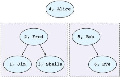
Before labeling the right subtree, you need to know how many elements you took from the stream when labeling the left subtree. Not only does the labeling function need to return the labeled tree, it also needs to return some information about where to start labeling the rest of the tree.
A natural way to do this might be for the labeling function to take the stream of labels as an input, as before, and to return a pair, containing
- The labeled tree
- A new stream of labels that you can use to label the rest of the tree
We’ll begin by implementing tree labeling this way, using a pair to represent the result of the operation and the state of the labels. Then, you’ll see how the State type defined in the Idris library encapsulates the state management details in this kind of algorithm.
12.1.2. Representing mutable state using a pair
Listing 12.3 defines a helper function to label a tree with a stream of labels, and uses a pair to represent the state of the stream after each subtree is labeled. The helper function returns the unused part of the stream of labels, so that when you’ve labeled one subtree, you know where to start labeling the next subtree.Listing 12.3. Labeling a Tree with a stream of labels (TreeLabel.idr)
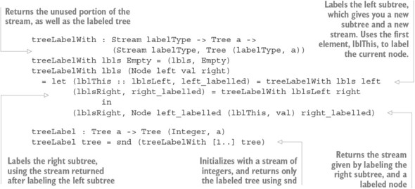
If you try labeling the example tree, you’ll see that the labels are applied in the order you expect:
*TreeLabel> flatten (treeLabel testTree) [(1, "Jim"), (2, "Fred"), (3, "Sheila"), (4, "Alice"), (5, "Bob"), (6, "Eve")] : List (Integer, String)
You can check that labeling also preserves the structure of the tree by omitting the call to flatten:
*TreeLabel> treeLabel testTree Node (Node (Node Empty (1, "Jim") Empty) (2, "Fred") (Node Empty (3, "Sheila") Empty)) (4, "Alice") (Node Empty (5, "Bob") (Node Empty (6, "Eve") Empty)) : Tree (Integer, String)
In the current definition of treeLabelWith, you need to keep track of the state of the stream of labels. Labeling a subtree not only gives you a tree with labels attached to the nodes, it also gives you a new stream of labels for labeling the next part of the tree.
As you traverse the tree, you keep track of the state of the stream by passing it as an argument, and returning the updated state. Essentially, the function uses local mutable state, with the state explicitly threaded through the definition. Although this works, there are two problems with this approach:- It’s error-prone because you need to ensure that the correct state is propagated correctly to the recursive calls. Notice that left_labelled and right_labelled have the same type, for example, so it’s easy to use the wrong one!
- It’s hard to read because the details of the algorithm are hidden behind the details of state management.
It’s often useful to have local mutable state, and like any concept you use regularly, it’s a good idea to create an abstraction that captures the concept. You can improve the definition of treeLabel, making it less error-prone and more readable, by using a type that captures the concept of state explicitly.
12.1.3. State, a type for describing stateful operations
The only reason you’re passing the stream of labels around in the definition of treeLabelWith is that when you encounter a value at a node, you need to associate it with a label value. In an imperative language, you might pass a mutable variable to tree-LabelWith and update it as you encounter each node. Because Idris is a purely functional language, you don’t have mutable variables, but the base library does provide a type for describing sequences of stateful operations, in the Control.Monad.State module. Control.Monad.State exports the following relevant definitions.
Listing 12.4. State and associated functions, defined in Control.Monad.State
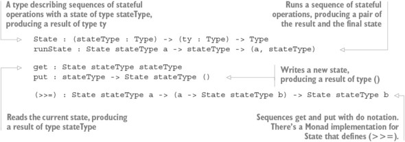
Just as a value of IO ty describes a sequence of interactive operations that produce a value of type ty, a value of type State Nat ty describes a sequence of operations that read and write a mutable state of type Nat. Listing 12.5 gives a small example of a function that works with mutable state. It reads the state using get and then updates it using put, increasing the Nat state by the given value.
Listing 12.5. A stateful function that increases a state by a given value (State.idr)
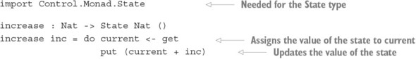
*State> runState (increase 5) 89 ((), 94) : ((), Nat)
The result is a pair of the value produced by the stateful operations, in this case the unit value (), and the final state, in this case 94. There are also two variants of runState:
- evalState—Returns only the value produced by the sequence of operations:
*State> :t evalState evalState : State stateType a -> stateType -> a *State> evalState (increase 5) 89 () : ()
- execState—Returns only the final state after the sequence of operations:
*State> :t execState execState : State stateType a -> stateType -> stateType *State> execState (increase 5) 89 94 : Nat
If you check the types of get and put, you’ll see that they use constrained generic types:
*TreeLabelState> :t get get : MonadState stateType m => m stateType *TreeLabelState> :t put put : MonadState stateType m => stateType -> m ()
This gives library authors more flexibility in defining stateful programs. The details of the MonadState interface are beyond the scope of this book, but you can read more in the Idris library documentation (http://idris-lang.org/documentation). In this example, you can read m as State stateType.
Although State encapsulates sequences of stateful operations, internally it’s defined using pure functions. Essentially, it encapsulates the implementation pattern you used to pass the state around in treeLabelWith.
12.1.4. Tree traversal with State
The next listing shows how you can define treeLabelWith by keeping the stream of labels as state, reading it to get the next label for a node.
Listing 12.6. Defining treeLabelWith as a sequence of stateful operations (TreeLabelState.idr)
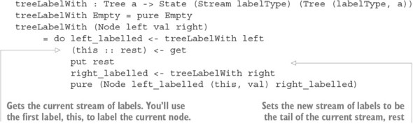
In this definition, you can see the details of the labeling algorithm more clearly than in the previous definition. Here, you leave the internal details of state management to the implementation of State.
In order to run this function and actually carry out the tree labeling, you’ll need to provide an initial state. The following listing defines a treeLabel function that initializes the state with an infinite stream of integers, counting upwards from 1.
Listing 12.7. Top-level function to label tree nodes, depth first, left to right (TreeLabelState.idr)

As before, you can test this at the REPL. It behaves the same way as the previous implementation of treeLabel on the test input:
*TreeLabelState> flatten (treeLabel testTree) [(1, "Jim"), (2, "Fred"), (3, "Sheila"), (4, "Alice"), (5, "Bob"), (6, "Eve")] : List (Integer, String)
Like IO, which you first encountered in chapter 5, State gives you a way of writing functions with side effects (here, modifying mutable state) by describing sequences of operations and executing them separately:
- A value of type IO ty is a description of a sequence of interactive actions producing a result of type ty. It’s executed by the runtime system by compilation, or by :exec at the REPL.
- A value of type State stateType ty is a description of a sequence of actions that read and write a state of type stateType, producing a result of type ty. It’s executed by using one of runState, execState, or evalState.
Many interesting programs follow this pattern, defining a type for describing sequences of commands and a separate function for executing those commands. Indeed, you’ve already seen one in chapter 11, when you defined the ConsoleIO type for describing indefinitely running interactive programs. You’ll see more examples in the remaining chapters, so in the rest of this chapter we’ll look at how to implement custom types for representing state and interaction.
Exercises
- Write a function that updates a state by applying a function to the current state:
update : (stateType -> stateType) -> State stateType ()
You should be able to use update to reimplement increase:increase : Nat -> State Nat () increase x = update (+x)
You can test your answer at the REPL as follows:*ex_12_1> runState (increase 5) 89 ((), 94) : ((), Nat)
- Write a function that uses State to count the number of occurrences of Empty in a tree. It should have the following type:
countEmpty : Tree a -> State Nat ()
You can test your answer at the REPL with testTree as follows:*ex_12_1> execState (countEmpty testTree) 0 7 : Nat
- Write a function that counts the number of occurrences of both Empty and Node in a tree, using State to store the count of each in a pair. It should have the following type:
countEmptyNode : Tree a -> State (Nat, Nat) ()
You can test your answer at the REPL with testTree as follows:*ex_12_1> execState (countEmptyNode testTree) (0, 0) (7, 6) : (Nat, Nat)
12.2. A custom implementation of State
In the previous section, you saw that the State type gives you a generic way of implementing algorithms that use state. You used it to maintain a stream of labels as local mutable state, which you could access by reading (using get) and writing (using put) as necessary. Like IO, which separates the description of an interactive program from its execution at runtime, State separates the description of a stateful program from its execution with a concrete state.We’ll look at more examples of the same pattern, separating the description of a program from its execution, in the remaining chapters, so before we go any further, let’s explore how we can define the State type ourselves, along with runState for executing stateful operations. In this section, you’ll see one way of defining State, and how to provide implementations of some interfaces for State: Functor, Applicative, and Monad. By implementing these interfaces, you’ll be able to use some generic library functions with State.
12.2.1. Defining State and runState
The following listing shows one way you could define State by hand, with a Get data constructor for describing the operation that reads state, and a Put data constructor for describing the operation that writes state.
Listing 12.8. A type for describing stateful operations (TreeLabelType.idr)
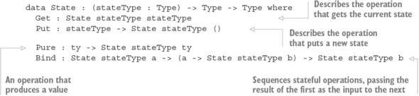
Remember that, by convention, type and data constructor names in Idris begin with a capital letter. I won’t deviate from this convention here, so if you want the same names as those exported by Control.Monad.State, you’ll need to define the following functions:
get : State stateType stateType get = Get put : stateType -> State stateType () put = Put pure : ty -> State stateType ty pure = Pure
(>>=) : State stateType a -> (a -> State stateType b) -> State stateType b (>>=) = Bind
Defining (>>=) means that you can use do notation for programs in State. As you saw in chapter 7, (>>=) is also a method of the Monad interface, which also requires implementations of the Functor and Applicative interfaces. It’s defined here as a standalone function to avoid the need to implement Functor and Applicative first for this example.
Where possible, it’s a very good idea to implement the Monad interface instead, because that gives you access to several constrained generic functions defined by the Idris library. For example, you’d be able to use the when function, which executes an operation when a condition is met, and traverse, which applies a computation across a structure. You’ll see how to do this for State in section 12.2.2.
Using this version of State, and defining the functions get, put, and pure, which directly use the data constructors, listing 12.9 shows how you can define treeLabelWith. This version is exactly the same as the previous one, as you’d expect, because it uses the same names for the functions that manipulate the state.
Listing 12.9. Defining treeLabelWith as a sequence of stateful operations (TreeLabelType.idr)
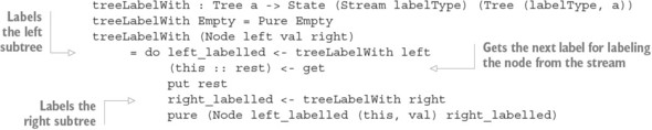
In order to run it, you’ll need to define a function that converts the description of the stateful operations into the tree-labeling function. The following listing shows the definition of runState, which takes a description of a stateful program and an initial state, and returns the value produced by the stateful program and a final state.
Listing 12.10. Running a labeling operation (TreeLabelType.idr)
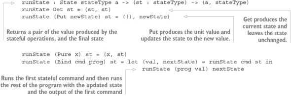
The following listing shows a definition of treeLabel that uses the new implementation of treeLabelWith, initializing the stream with [1..].
Listing 12.11. The tree-labeling function, which calls run with an initial stream of labels (TreeLabelType.idr)

12.2.2. Defining Functor, Applicative, and Monad implementations for State
Implementing (>>=) for State means that you can use do notation, which gives a clear, readable notation for writing functions that describe sequences of operations. But do notation is all it gives us.
Rather than defining (>>=) as a standalone function, it’s a good idea to implement the Functor, Applicative, and Monad interfaces for State. In addition to providing do notation via the Monad interface, this will give you access to generic functions defined in the library. For example, when and traverse are generic functions. In the context of IO, they behave as follows:
- when evaluates a computation if a condition is True. It could be used to run some IO actions only on a specific user input.
- traverse is similar to map and applies a computation across a structure. For example, you could print every element of a List to the console.
You can find out more about these functions, especially their types, with :doc. The following listing shows them in action in the context of an IO computation.
Listing 12.12. Using when and traverse (Traverse.idr)
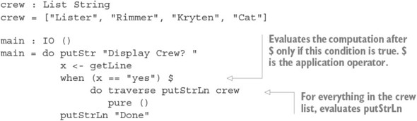
when (x == "yes") (do traverse putStrLn crew pure ())
If you implement Functor, Applicative, and Monad for State, you’ll be able to use these and other similar functions in functions that use State. The next listing shows an example of what you can do, giving a function that adds Integers from a list to a running total, provided the Integer is positive. At the moment, this will fail to type-check.
Listing 12.13. Adding positive integers from a list to a state (StateMonad.idr)
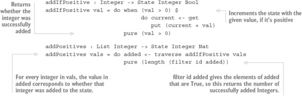
This will fail because you don’t have implementations of Functor or Applicative for State:
StateMonad.idr:42:15: When checking right hand side of addIfPositive with expected type State Integer Bool When checking an application of function Main.>>=: Can't find implementation for Applicative (State Integer)Your ultimate goal here is to implement Monad for State, which also requires implementations of Functor and Applicative. The next listing shows the Monad interface, as defined in the Prelude.
Listing 12.14. The Monad interface
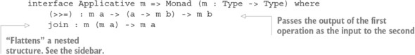
We haven’t looked at join in detail, but you can use it to flatten nested structures into a single structure. For example, there are implementations of Monad for List and Maybe, so you can try join on examples of each:
Idris< join [[1,2,3], [4,5,6]] [1, 2, 3, 4, 5, 6] : List Integer Idris< join (Just (Just "One")) Just "One" : Maybe String Idris< join (Just (Nothing {a=String})) Nothing : Maybe String For List, join will concatenate the nested lists. For Maybe, join will find the single value nested in the structure, if any.
Both methods, (>>=) and join, have default definitions, so you can implement Monad by defining one or both of these. Here, we’ll only use (>>=).
If you want to provide an implementation for Monad, you also need to implement Applicative, because it’s a parent interface of Monad. Similarly, Applicative has a parent interface, Functor. The following listing shows both interfaces as defined in the Prelude.
Listing 12.15. The Functor and Applicative interfaces
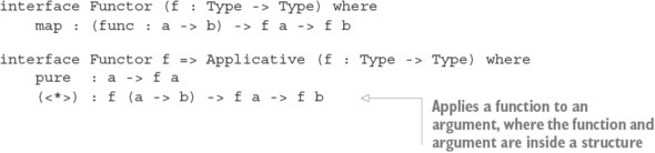
The (<*>) method allows you to, for example, have a stateful function that returns a function (of type a -> b), have another stateful function that returns an argument (of type a), and apply the function to the argument.
You can begin by implementing Functor as follows:
- Type, define—Write the implementation header and create a skeleton definition of map. Remember that you can create skeleton definitions for interface methods by pressing Ctrl-Alt-A with the cursor over the interface name:
Functor (State stateType) where map func x = ?Functor_rhs_1
- Type, refine—The type of the ?Functor_rhs_1 hole tells you that x is a stateful computation:
stateType : Type b : Type a : Type func : a -> b x : State stateType a -------------------------------------- Functor_rhs_1 : State stateType b
You can continue the definition by extracting the value from the computation x using Bind:Functor (State stateType) where map func x = Bind x (\val => ?Functor_rhs_1)
- Refine— To complete the definition, pass val to func, and use Pure to convert the result to a stateful computation:
Functor (State stateType) where map func x = Bind x (\val => Pure (func val))
Listing 12.16 shows the definitions of Applicative and Monad for State. You implement Applicative in a way similar to Functor, using Bind to extract the values you need from stateful computations.
Listing 12.16. Implementing Applicative and Monad for State (StateMonad.idr)
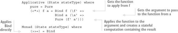
You’ve used Bind in the implementations of Functor and Applicative because you don’t have do notation available yet. You need a Monad implementation to provide it,
and you need to have Functor and Applicative implementations to have a Monad implementation.But you could use do notation by defining all the implementations together, in a mutual block, as listing 12.17 shows. In a mutual block, definitions can refer to each other, so the implementations of Functor and Applicative can rely on the implementation of Monad.
Listing 12.17. Defining Functor, Applicative, and Monad implementations together (StateMonad.idr)
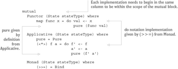
Now that you’ve implemented these interfaces, you can try the earlier definition of addPositives from listing 12.13:
*StateMonad> runState (addPositives [-4, 3, -8, 9, 8]) 0 (3, 20) : (Nat, Integer)
Given that you have Monad implementations for State and IO, sequencing stateful computations and interactive computations respectively, it’s reasonable to wonder whether you can sequence both at once, in the same function—what about interactive programs that also manipulate state?
You’ll see one way to do this in the next section. As a more general solution, though, Idris provides a library called Effects that supports combining different kinds of side effects like State and IO in types, as well as other effects such as exceptions and nondeterminism. You can find more details in the Effects library tutorial (http://idris-lang.org/documentation/effects).
You’ve now seen how to encapsulate the details of state manipulation by describing sequences of stateful operations as State, and executing them using runState. You’ve also seen how to implement Functor, Applicative, and Monad for State.
The states you’ve used in the examples so far have been fairly small: a single stream of labels, or a single Integer. More generally, state can get fairly complex:- State may consist of several complex components, stored as a record. We’ll discuss this in the rest of this chapter, where you’ll see how to write a complete interactive program with state.
- You might want to use a dependent type in your State, in which case updating the state will also update its type! For example, if you add an element to a Vect 8 Int, it would become a Vect 9 Int. We’ll discuss this in the next chapter.
An advantage of writing a type that expresses sequences of commands, along with a function for running those commands, is that you can make the command type as precise as you need. As you’ll see in the next section, you can describe precisely the set of commands you need for a specific application, including commands for interaction at the console and commands for reading and writing components of the application’s state. In the next chapter, you’ll see how you can precisely describe in its type the effect each command has on a system’s state.
12.3. A complete program with state: working with records
In the previous chapter, you implemented an arithmetic quiz that presented multiplication problems to the user and kept track of the numbers of correct answers and questions asked. In this section, we’ll write a refined version, with the following improvements:
- We’ll add a difficulty setting, which specifies the largest number allowed when generating questions.
- Instead of passing the current score as an argument to the quiz function, maintaining the state by hand, we’ll extend the Command type with commands for giving access to the current score and the difficulty setting.
To write this refined version, we’ll need to rethink how to represent the game’s state. We’ll do this using record types. You’ve already seen some the use of records to represent the data store in chapter 6, with similar examples in chapters 7 and 10. As an application’s state grows, though, it can make sense to divide its state into several hierarchical records.
You’ll see how to define and use nested records, how to update records with a concise syntax, and how to use a record to store the state of the interactive quiz program. First, though, we’ll revisit the Command type from chapter 11 and see how you can extend it to support reading and writing system state, in a way similar to the custom State type defined in the previous section.
12.3.1. Interactive programs with state: the arithmetic quiz revisited
In chapter 11, you defined a Command data type, representing the commands you could use in console I/O programs, and a ConsoleIO type, representing possibly infinite interactive processes. You used this to implement an arithmetic quiz, presenting
multiplication problems for a user to answer. Like State, which describes the operations Get and Put for reading and writing state, Command describes the operations GetLine and PutStr for reading from and writing to the console. The following listing recaps the definitions of Command and ConsoleIO.Listing 12.18. Interactive programs supporting only console I/O (ArithState.idr)
Implementing Monad for Command
As with State, you could implement Functor, Applicative, and Monad for Command instead of implementing (>>=) directly. As an exercise, try providing implementations of each. As I noted in the last chapter, however, you can’t provide a Monad implementation for ConsoleIO because the type of ConsoleDo.(>>=) doesn’t fit.
Like runState, which takes a description of stateful operations and returns the result of executing those operations with an initial state, run takes a description of interactive operations and executes them in IO. Listing 12.19 recaps the run function. Remember that you limit how long interactive programs can run by using the Fuel type, and you add a nontotal function, forever, that allows a total interactive program to run indefinitely, while only introducing a single nontotal function.
Listing 12.19. Running interactive programs (ArithState.idr)
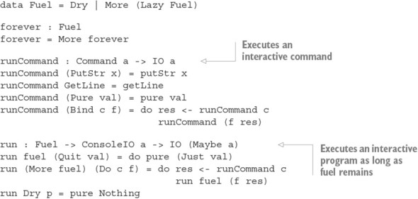
- Get random numbers for the questions, given the game’s difficulty setting.
- Read the current game state so that you can display the score.
- Update the game state so that you can update the score according to the user’s answers.
The next listing shows how you can extend the Command data type to include these commands. There’s no need to update ConsoleIO, because it merely sequences Commands.
Listing 12.20. Extending the Command type to support game state (ArithState.idr)
GameState is undefined for the moment, so you can’t yet complete run or run-Command. You can, however, add pattern clauses with holes for the extra commands so that the totality checker is satisfied:
runCommand : Command a -> IO a runCommand (PutStr x) = putStr x runCommand GetLine = getLine runCommand (Pure val) = pure val runCommand (Bind c f) = do res <- runCommand c runCommand (f res) runCommand (PutGameState x) = ?runCommand_rhs_1 runCommand GetGameState = ?runCommand_rhs_2 runCommand GetRandom = ?runCommand_rhs_3
Adding missing cases
After you’ve added constructors to Command, you can use Ctrl-Alt-A with the cursor over runCommand in the type declaration to add the new pattern clauses for runCommand.
12.3.2. Complex state: defining nested records
In the refined quiz implementation, you’ll use GameState to store the following:
- The current score, consisting of the number of questions answered correctly and the number attempted
- The difficulty setting
When there are several components to a program’s state like this, it often makes sense to use a record type. Records are convenient because they give rise to projection functions, which allow you to inspect the fields of the record. You can also nest records; the following listing shows how you can represent the current score as a record, and the overall game state as a record, including the nested score record as a field.
Listing 12.21. Representing a game state as nested records (ArithState.idr)
Defining Score and GameState as records automatically generates projection functions for each field: correct, attempted, score, and difficulty. For example, you can get the difficulty level like this:
*ArithState> difficulty initState 12 : Int
Or you can get the number of correct answers so far:
*ArithState> correct (score initState) 0 : Nat
When you define a record, the projection functions are defined in their own name-space, given by the name of the record. For example, the score function is defined in a new GameState namespace, as you can see with :doc at the REPL:
*ArithState> :doc score Main.GameState.score : (rec : GameState) -> ScoreThis allows the same field name to be used multiple times within the same module. For example, you can use a field called title in two different records in the same file, Record.idr:
record Book where constructor MkBook title : String author : String record Album where constructor MkAlbum title : String tracks : List String
Idris will decide which version of title to use, according to context:
*Record> title (MkBook "Breakfast of Champions" "Kurt Vonnegut") "Breakfast of Champions" : String
The following listing shows how you can use projection functions to define an implementation of Show for GameState.
Listing 12.22. Show implementation for GameState (ArithState.idr)
Show GameState where show st = show (correct (score st)) ++ "/" ++ show (attempted (score st)) ++ "\n" ++ "Difficulty: " ++ show (difficulty st)
You can try this at the REPL, using printLn to display the initial game state:
*ArithState> :exec printLn initState 0/0 Difficulty: 12
Records, therefore, give you a convenient notation for inspecting field values, but when you write programs that use records to hold state, you’ll also need to update fields. In the quiz, for example, you’ll need to increment the score and the number of questions attempted.
12.3.3. Updating record field values
Idris is a pure functional language, so you won’t update record fields in-place. Instead, when we say we’re updating a record, we really mean that we’re constructing a new record containing the contents of the old record with a single field changed. For example, the following listing shows one way to return a new record with the difficulty field updated, using pattern matching.
Listing 12.23. Setting a record field by pattern matching (ArithState.idr)
setDifficulty : Nat -> GameState -> GameState setDifficulty newDiff (MkGameState score _) = MkGameState score newDiffIf the record has a lot of fields, this can get unwieldy very quickly, because you’d need to write update functions for every field. Not only that, if you were to add a field to a record, you’d need to modify all of the update functions. Idris therefore provides a built-in syntax for updating fields in records. Here’s an implementation of setDifficulty using record-update syntax.
Listing 12.24. Setting a record field using record-update syntax (ArithState.idr)
setDifficulty : Nat -> GameState -> GameState setDifficulty newDiff state = record { difficulty = newDiff } state Figure 12.3 shows the components of the record-update syntax. Note in particular that the record-update syntax itself is first-class, where record is a keyword that begins a record update, so the record update has a type. Here, the update has a function type, GameState -> GameState, so you can also implement setDifficulty as follows:
setDifficulty : Nat -> GameState -> GameState setDifficulty newDiff = record { difficulty = newDiff } Figure 12.3. Syntax for returning a new record with a field updated
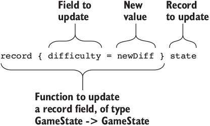
You can update nested record fields in a similar way, by giving the path to the field you’d like to update. The following listing shows how you can write the correct and wrong functions, which update the score.
Listing 12.25. Setting nested record fields using record-update syntax (ArithState.idr)
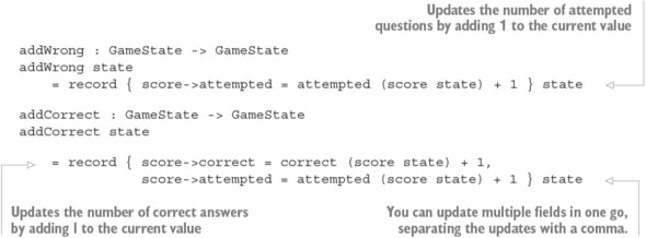
12.3.4. Updating record fields by applying functions
The record-update syntax offers a concise notation for specifying a path to a particular record field. It’s still a little inconvenient, though, because you’ve needed to explicitly write the path to each field twice, in different notations:
- First, to find the field to update, using the score->correct path notation
- Second, to find the old value, using a function application, correct (score state)
Idris therefore provides a notation for updating record fields by directly applying a function to the current value of the field. The next listing shows a concise way of updating the nested record fields in GameState.
Listing 12.26. Updating nested record fields by directly applying functions to the current value of the field (ArithState.idr)
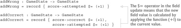
Updating records with $=
You saw the $ operator, which applies a function to an argument, in chapter 10. The $= syntax arises from a combination of the function application operator $ and the record-update syntax.
This syntax gives you a concise and convenient way of writing functions that update nested record fields, which makes it easier to write programs that manipulate state. Moreover, because it doesn’t use pattern matching, it’s independent of any other fields in a record, so even if you add fields to the GameState record, addWrong and addCorrect will work without modifications.
12.3.5. Implementing the quiz
Using your new Command type and the GameState record, you can implement the arithmetic quiz by reading and updating the state as necessary. The next listing shows an outline of the quiz implementation, leaving holes for correct and wrong, which, respectively, process a correct answer and a wrong answer.
Listing 12.27. Implementing the arithmetic quiz (ArithState.idr)
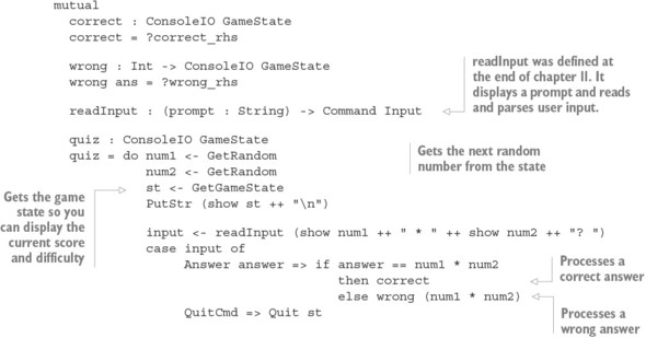
This is similar to the implementation of quiz at the end of chapter 11, but instead of passing the stream of random numbers and the score as arguments, you treat each of them as state that you read and write as required. This simplifies the definition of quiz, at the cost of making the definition of ConsoleIO more complex.
The next listing shows how you can implement correct and wrong, each modifying the state using addCorrect and addWrong, respectively, as defined in the previous section.
Listing 12.28. Processing correct and wrong answers by updating the game state (ArithState.idr)
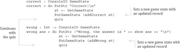
At this stage, you have a complete description of an interactive arithmetic quiz that retrieves random numbers and the current score from the state. It’s also total:
*ArithState> :total quiz Main.quiz is TotalBut to run quiz, you’ll need to extend runCommand to support your new commands.
12.3.6. Running interactive and stateful programs: executing the quiz
As with the runState function you wrote for processing operations in the custom State type in section 12.2, the updated run function will need to process the current game state. It will also need to read from a stream of random numbers (for Get-Random) and perform console I/O. The following listing shows how these are all captured in a new type for runCommand.
Listing 12.29. A new type and skeleton definition for runCommand (ArithState.idr)
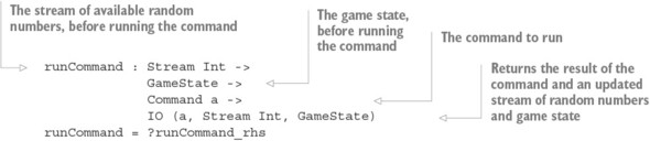
Listing 12.30 gives the complete definition of runCommand. Note that, in each case, you need to return the result of the command as well as show how each command affects the random number stream and the game state.
Listing 12.30. The complete definition of runCommand (ArithState.idr)

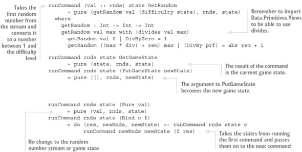
Similarly, you need to update run to take a stream of random integers and an initial game state. Like runCommand, run also returns the result of running the program, along with the updated stream and game state. Here’s the new implementation of run, which supports the game state.
Listing 12.31. Running a ConsoleIO program consisting of a potentially infinite stream of Command (ArithState.idr)
run : Fuel -> Stream Int -> GameState -> ConsoleIO a -> IO (Maybe a, Stream Int, GameState) run fuel rnds state (Quit val) = do pure (Just val, rnds, state) run (More fuel) rnds state (Do c f) = do (res, newRnds, newState) <- runCommand rnds state c run fuel newRnds newState (f res) run Dry rnds state p = pure (Nothing, rnds, state)
As in chapter 11, you use Fuel to say how long you’re willing to allow a potentially infinite interactive program to run, so the portion of the return type that represents the result of running the program, of type ConsoleIO a, has type Maybe a, to capture the possibility of running out of Fuel.
Finally, the next listing shows how you update the main program to initialize the stream of random numbers and the game state.
Listing 12.32. A main program that initializes the arithmetic quiz with a random number stream and an initial state (ArithState.idr)
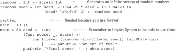
As with the implementation of quiz at the end of chapter 11, you separate terminating sequences of commands (using the Command type) from possible nonterminating sequences of console I/O operations (using the ConsoleIO type). In addition, you extend the Command type to allow reading and writing of the game’s state much like
the implementation of State. If you define a specific type for the commands that an application can execute, you can make that type as precise as you need, possibly describing the effect of each operation on an abstraction of a system’s state. You’ll see more of what you can achieve by following this pattern and the guarantees you can make about stateful, interactive programs in the next chapter.Exercises
- Write an updateGameState function with the following type:
updateGameState : (GameState -> GameState) -> Command ()
You can test it by using it in the definitions of correct and wrong instead of GetGameState and PutGameState. For example:correct : ConsoleIO GameState correct = do PutStr "Correct!\n" updateGameState addCorrect quiz
- Implement the Functor, Applicative, and Monad interfaces for Command.
- You could define records for representing an article on a social news website as follows, along with the number of times the article has been upvoted or downvoted:
record Votes where constructor MkVotes upvotes : Integer downvotes : Integer record Article where constructor MkArticle title : String url : String score : Votes initPage : (title : String) -> (url : String) -> Article initPage title url = MkArticle title url (MkVotes 0 0)
Write a function to calculate the overall score of a given article, where the score is calculated from the number of downvotes subtracted from the number of upvotes. It should have the following type:getScore : Article -> Integer
You can test it with the following example articles:badSite : Article badSite = MkArticle "Bad Page" "http://example.com/bad" (MkVotes 5 47) goodSite : Article goodSite = MkArticle "Good Page" "http://example.com/good" (MkVotes 101 7)
At the REPL, you should see the following:*ex_12_3> getScore goodSite 94 : Integer *ex_12_3> getScore badSite -42 : Integer
- Write addUpvote and addDownvote functions that modify an article’s score up or down. They should have the following types:
addUpvote : Article -> Article addDownvote : Article -> Article
You can test these at the REPL as follows:*ex_12_3> addUpvote goodSite MkArticle "Good Page" "http://example.com/good" (MkVotes 102 7) : Article *ex_12_3> addDownvote badSite MkArticle "Bad Page" "http://example.com/bad" (MkVotes 5 48) : Article *ex_12_3> getScore (addUpvote goodSite) 95 : Integer
12.4. Summary
- Many algorithms read and write state. For example, when labeling the nodes of a tree in depth-first order, you can keep track of the state of the labels while traversing the tree.
- You can manage state by using the generic State type to describe operations on the state along with a runState function to execute those operations.
- You can define your own State type as a sequence of Get and Put operations.
- Defining Functor, Applicative, and Monad for the State type gives you access to several generic functions from the Idris library.
- When writing interactive programs with state, you can define a Command type to describe an interface consisting of console I/O and state management operations.
- Record types can represent more complex nested state.
- Idris provides a concise syntax for assigning new values to fields in nested records.
- Idris also provides a syntax (using $=) for updating a field in a nested record by applying a function to the value in that field.
Chapter 13. State machines: verifying protocols in types
This chapter covers
- Specifying protocols in types
- Describing preconditions and postconditions of operations
- Using dependent types in state
In the previous chapter, you saw how to manage mutable state by defining a type for representing sequences of commands in a system, and a function for running those commands. This follows a common pattern: the data type describes a sequence of operations, and the function interprets that sequence in a particular context. For example, State describes sequences of stateful operations, and runState interprets those operations with a specific initial state.
In this chapter, we’ll look at one of the advantages of using a type for describing sequences of operations and keeping the execution function separate. It allows you to make the descriptions more precise, so that certain operations can only be run when the state has a specific form. For example, some operations require access to a resource, such as a file handle or database connection, before they’re executed:
- You need an open file handle to read from a file successfully.
- You need a connection to a database before you can run a query on the database.
When you write programs that work with resources like this, you’re really working with a state machine. A database client might have two states, such as Closed and Connected, referring to its connection status to a database. Some operations (such as querying the database) are only valid in the Connected state; some (such as connecting to the database) are only valid in the Closed state; and some (such as connecting and closing) also change the state of the system. Figure 13.1 illustrates this system.
Figure 13.1. A state transition diagram showing the high-level operation of a database. It has two possible states, Closed and Connected. Its three operations, Connect, Query, and Close, are only valid in specific states.
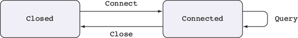
State machines like the one illustrated in figure 13.1 exist, implicitly, in lots of real-world systems. When you’re implementing communicating systems, for example, whether over a network or using concurrent processes, you need to make sure each party is following the same communication pattern, or the system could deadlock or behave in some other unexpected way. Each party follows a state machine where sending or receiving a message puts the overall system into a new state, so it’s important that each party follows a clearly defined protocol. In Idris, we have an expressive type system, so if there’s a model for a protocol, it’s a good idea to express that in a type, so that you can use the type to help implement the protocol accurately.
In this chapter, you’ll see how to make state machines like the one illustrated in figure 13.1explicit in types. In this way, you can be sure that any function that correctly describes a sequence of actions follows the protocol defined by a state machine. Not only that, you can take a type-driven approach to defining sequences of actions using holes and interactive development. We’ll begin with some fairly abstract examples to illustrate how you can describe state machines in types, modeling the states and operations on a door and a vending machine.
13.1. State machines: tracking state in types
You’ve previously implemented programs with state by defining a type that describes commands for reading and writing state. With dependent types, you can make the types of these commands more precise and include any relevant details about the state of the system in the type itself.
For example, let’s consider how to represent the state of a door with a doorbell. A door can be in one of two states, open (represented as DoorOpen) or closed (represented as DoorClosed), and we’ll allow three operations:
- Opening the door, which moves the system from the DoorClosed state to the DoorOpen state
- Closing the door, which moves the system from the DoorOpen state to the DoorClosed state
- Ringing the doorbell, which we’ll only allow when the door is in the DoorClosed state
Figure 13.2 is a state transition diagram that shows the states the system can be in and how each operation modifies the overall state.
Figure 13.2. A state transition diagram showing the states and operations on a door
If you can define these state transitions in a type, then a well-typed description of a sequence of operations must correctly follow the rules shown in the state transition diagram. Furthermore, you’ll be able to use holes and interactive editing to find out which operations are valid at a particular point in a sequence.
In this section, you’ll see how to define state machines like the door in a dependent type. First, we’ll implement a model of the door, and then we’ll model more-complex states in a model of a simplified vending machine. In each case, we’ll focus on the model of the state transitions, rather than a concrete implementation of the machine.
13.1.1. Finite state machines: modeling a door as a type
The state machine in figure 13.2 describes a protocol for correct use of a door by saying which operations are valid in which state, and how those operations affect the state. Listing 13.1 shows one way to represent the possible operations. This also includes a (>>=) constructor for sequencing and a Pure constructor for producing pure values.
Listing 13.1. Representing operations on a door as a command type (Door.idr)
Reminder: (>>=) and do notation
Remember that do notation translates into applications of (>>=).
doorProg : DoorCmd () doorProg = do RingBell Open Close
Unfortunately, you can also describe invalid sequences of operations that don’t follow the protocol, such as the following, where you attempt to open a door twice, and then ring the doorbell when the door is already open:
doorProgBad : DoorCmd () doorProgBad = do Open Open RingBell
You can avoid this, and limit functions with DoorCmd to valid sequences of operations that do follow the protocol, by keeping track of the door’s state in the type of the DoorCmd operations. The following listing shows how to do this, describing exactly the state transitions represented in figure 13.2 in the types of the commands.
Listing 13.2. Modeling the door state machine in a type, describing state transitions in the types of the commands (Door.idr)
Each command’s type takes three arguments:
- The type of the value produced by the command
- The input state of the door; that is, the state the door must be in before you can execute the operation
- The output state of the door; that is, the state the door will be in after you execute the operation
doorProg : DoorCmd () DoorClosed DoorClosed
Argument order in DoorCmd
Notice that the type that a sequence of operations produces is the first argument to DoorCmd, and it’s followed by the input and output states. This is a common convention when defining types for describing state transitions, and it will become important in chapter 14 when we look at more-complex state machines that deal with errors and feedback from the environment.
In general, if you have a value of type DoorType ty beforeState afterState, it describes a sequence of door actions that produces a value of type ty; it begins with the door in the state beforeState; and it ends with the door in the state afterState.
13.1.2. Interactive development of sequences of door operations
To see how the types in DoorCmd can help you write sequences of operations correctly, let’s reimplement doorProg. We’ll write this in the same way as before: ring the doorbell, open the door, and close the door.
If you write it incrementally, you’ll see how the type shows the changes in the state of the door throughout the sequence of actions:
- Define— Begin with the skeleton definition:
doorProg : DoorCmd () DoorClosed DoorClosed doorProg = ?doorProg_rhs
- Refine, type—Add an action to ring the doorbell:
doorProg : DoorCmd () DoorClosed DoorClosed doorProg = do RingBell ?doorProg_rhs
If you check the type of ?doorProg_rhs now, you’ll see that it should be a sequence of actions that begins and ends with the door in the DoorClosed state:-------------------------------------- doorProg_rhs : DoorCmd () DoorClosed DoorClosed
- Refine, type—Next, add an action to open the door:
doorProg : DoorCmd () DoorClosed DoorClosed doorProg = do RingBell Open ?doorProg_rhs
If you check the type of ?doorProg_rhs now, you’ll see that it should begin with the door in the DoorOpen state instead:-------------------------------------- doorProg_rhs : DoorCmd () DoorOpen DoorClosed
- Refine failure—If you add an extra Open now, with the door already in the DoorOpen state, you’ll get a type error:
doorProg : DoorCmd () DoorClosed DoorClosed doorProg = do RingBell Open Open ?doorProg_rhs
The error says that the type of Open is an operation that starts in the DoorClosed state, but the expected type starts in the DoorOpen state:Door.idr:20:15: When checking right hand side of doorProg with expected type DoorCmd () DoorClosed DoorClosed When checking an application of constructor Main.>>=: Type mismatch between DoorCmd () DoorClosed DoorOpen (Type of Open) and DoorCmd a DoorOpen state2 (Expected type) Specifically: Type mismatch between DoorClosed and DoorOpen
- Refine— Instead, complete the definition by closing the door:
doorProg : DoorCmd () DoorClosed DoorClosed doorProg = do RingBell Open Close
The type of doorProg includes input and output states that give preconditions and postconditions for the sequence (the door must be closed both before and after the sequence). If the definition violates either, you’ll get a type error.
For example, you might forget to close the door:
doorProg : DoorCmd () DoorClosed DoorClosed doorProg = do RingBell Open
In this case, you’ll get a type error:
Door.idr:18:15: When checking right hand side of doorProg with expected type DoorCmd () DoorClosed DoorClosed When checking an application of constructor Main.>>=: Type mismatch between DoorCmd () DoorClosed DoorOpen (Type of Open) and DoorCmd () DoorClosed DoorClosed (Expected type) Specifically: Type mismatch between DoorOpen and DoorClosedThe error refers to the final step and says that Open moves from DoorClosed to DoorOpen, but the expected type is to move from DoorClosed to DoorClosed.
By defining DoorCmd in this way, with the input and output states explicit in the type, you’ve defined what it means for a sequence of door operations to be valid. And by writing doorProg incrementally, with a sequence of steps and a hole for the rest of the definition, you can see the state of the door at each stage by looking at the type of the hole.
The door has exactly two states, DoorClosed and DoorOpen, and you can describe exactly when you change states from one to the other in the types of the door operations. But not all systems have an exact number of states that you can determine in advance. Next, we’ll look at how you can model systems with an infinite number of possible states.
13.1.3. Infinite states: modeling a vending machine
In this section, we’ll model a vending machine using type-driven development, writing types that explicitly describe the input and output states of each operation. As a simplification, the machine accepts only one type of coin (a £1 coin) and dispenses one product (a chocolate bar). Even so, there could be an arbitrarily large number of coins or chocolate bars in the machine, so the number of possible states is not finite.
Table 13.1 describes the basic operations of a vending machine, along with the state of the machine before and after each operation.
Table 13.1. Vending machine operations, with input and output states represented as Nat
| Coins (before) | Chocolate (before) | Operation | Coins (after) | Chocolate (after) |
|---|---|---|---|---|
| pounds | chocs | Insert coin | S pounds | chocs |
| S pounds | S chocs | Vend chocolate | pounds | chocs |
| pounds | chocs | Return coins | Z | chocs |
As with the door example, each operation has a precondition and a postcondition:
- Precondition— The number of coins and amount of chocolate that must be in the machine before the operation
- Postcondition— The number of coins and amount of chocolate in the machine after the operation.
You can represent the state of the machine as a pair of two Nats, the first representing the number of coins in the machine and the second representing the number of chocolates:
VendState : Type VendState = (Nat, Nat)
The next listing shows a representation of the vending machine state as an Idris type, with the state transitions from table 13.1 explicitly written in the types of the MachineCmd operations.
Listing 13.3. Modeling the vending machine in a type, describing state transitions in the types of commands (Vending.idr)
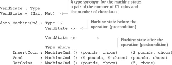
To complete the model, you’ll need to be able to sequence commands. You’ll also need to be able to read user input: the commands you’re defining describe what the machine does, but there’s also a user interface that consists of the following:
- A coin slot
- A vend button, for dispensing chocolate
- A change button, for returning any unused coins
You can model these operations in a data type for describing possible user inputs. Listing 13.4 shows the complete model of the vending machine, including additional operations for displaying a message (Display), refilling the machine (Refill), and reading user actions (GetInput).
Listing 13.4. The complete model of vending machine state (Vending.idr)
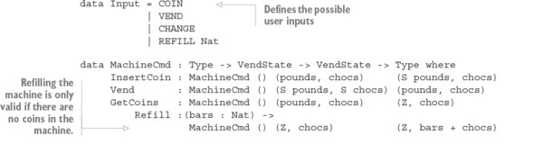
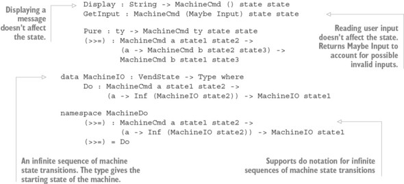
13.1.4. A verified vending machine description
Listing 13.5 shows the outline of a function that describes verified sequences of operations for a vending machine using the state transitions defined by MachineCmd. As long as it type-checks, you know that you’ve correctly sequenced the operations, and you’ll never execute an operation without its precondition being satisfied.Listing 13.5. A main loop that reads and processes user input to the vending machine (Vending.idr)
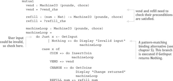
There are holes for vend and refill. In each case, you need to check that the number of coins and chocolates satisfy their preconditions. If you try to Vend without checking the precondition, Idris will report an error:
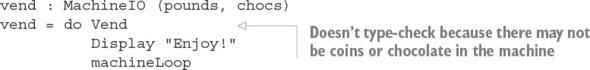
Idris will report an error because you haven’t checked whether there’s a coin in the machine and a chocolate bar available, so the precondition might not be satisfied:
Vending.idr:67:13: When checking right hand side of vend with expected type MachineIO (pounds, chocs) When checking an application of function Main.MachineDo.>>=: Type mismatch between MachineCmd () (S pounds1, S chocs2) (pounds1, chocs2) (Type of Vend) and MachineCmd () (pounds, chocs) (pounds1, chocs2) (Expected type) Specifically: Type mismatch between S chocs1 and chocs
The error says that the input state must be of the form (S pounds1, S chocs2), but instead it’s of the form (pounds, chocs).
You can solve this problem by pattern matching on the implicit arguments, pounds and chocs, to ensure they’re in the right form, or display an error otherwise. The following listing shows definitions of vend and refill that do this.
Listing 13.6. Adding definitions of vend and refill that check that their preconditions are satisfied (Vending.idr)
In the next section, you’ll see a more concrete example of tracking state in the type, implementing a stack data structure. I’ll use this example to illustrate how you can execute commands in practice.
Exercises
- Change the RingBell operation so that it works in any state, rather than only when the door is closed. You can test your answer by seeing that the following function type-checks:
doorProg : DoorCmd () DoorClosed DoorClosed doorProg = do RingBell Open RingBell Close
- The following (incomplete) type defines a command for a guessing game, where the input and output states are the number of remaining guesses allowed:
data GuessCmd : Type -> Nat -> Nat -> Type where Try : Integer -> GuessCmd Ordering ?in_state ?out_state Pure : ty -> GuessCmd ty state state (>>=) : GuessCmd a state1 state2 -> (a -> GuessCmd b state2 state3) -> GuessCmd b state1 state3
The Try command returns an Ordering that says whether the guess was too high, too low, or correct, and that changes the number of available guesses. Complete the type of Try so that you can only make a guess when there’s at least one guess allowed, and so that guessing reduces the number of guesses available. If you have a correct answer, the following definition should type-check:threeGuesses: GuessCmd () 3 0 threeGuesses = do Try 10 Try 20 Try 15 Pure ()
Also, the following definition shouldn’t type-check:noGuesses : GuessCmd () 0 0 noGuesses = do Try 10 Pure ()
- The following type defines the possible states of matter:
data Matter = Solid | Liquid | Gas
Define a MatterCmd type in such a way that the following definitions type-check:iceSteam : MatterCmd () Solid Gas iceSteam = do Melt Boil steamIce : MatterCmd () Gas Solid steamIce = do Condense Freeze
Additionally, the following definition should not type-check:overMelt : MatterCmd () Solid Gas overMelt = do Melt Melt
13.2. Dependent types in state: implementing a stack
You’ve seen how to model state transitions in a type for two abstract examples: a door (representing whether it was open or closed in its type) and a vending machine (representing its contents in its type). Storing this abstract information in the type of the operations is particularly useful when you also have concrete data that relates to that abstract data. For example, if you’re describing data of a specific size, and the type of an operation tells you how it changes the size of the data, you can use a Vect as a concrete representation. You’ll know the required length of the input and output Vect from the type of each operation.
In this section, you’ll see how this works by implementing operations on a stack data structure. A stack is a last-in, first-out data structure where you can add items to and remove them from the top of the stack, and only the top item is ever accessible. A stack supports three operations:
- Push—Adds a new item to the top of the stack
- Pop—Removes the top item from the stack, provided that the stack isn’t empty
- Top—Inspects the top item on the stack, provided that the stack isn’t empty
Like the operations on the vending machine, each of these operations has a precondition that describes the necessary input state and a postcondition describing the output state. Table 13.2 describes these, giving the required stack size before each operation and the resulting stack size after the operation.
Table 13.2. Stack operations, with input and output stack sizes represented as Nat
| Stack size (before) | Operation | Stack size (after) |
|---|---|---|
| height | Push element | S height |
| S height | Pop element | height |
| S height | Inspect top element | S height |
You’ll express the preconditions and postconditions in the types of each operation. Once you’ve defined the operations on a stack, you’ll implement a function to run sequences of stack operations using a concrete representation of a stack with its height in its type. Because you’re using the stack’s height in the state transitions, a good concrete representation of a stack is a Vect. You know, for example, that a stack of Integer of height 10, contains exactly 10 integers, so you can represent this as a value of type Vect 10 Integer.
Finally, you’ll see an example of a stack in action, implementing a stack-based interactive calculator.
13.2.1. Representing stack operations in a state machine
As with DoorCmd and MachineCmd in section 13.1, we’ll describe operations on a stack in a dependent type and put the important properties of the input and output states explicitly in the type. Here, the property of the state that interests us is the height of the stack.
Listing 13.7 shows how you can express the operations in table 13.2 in code, describing how each operation affects the height of the stack. For this example, you’ll only store Integer values on the stack, but you could extend StackCmd to allow generic stacks by parameterizing over the element type in the stack.
Listing 13.7. Representing operations on a stack data structure with the input and output heights of the stack in the type (Stack.idr)
Using StackCmd, you can write sequences of stack operations where the input and output heights of the stack are explicit in the types. For example, the following function pushes two integers, pops two integers, and then returns their sum:
testAdd : StackCmd Integer 0 0 testAdd = do Push 10 Push 20 val1 <- Pop val2 <- Pop Pure (val1 + val2)
The types of the constructors in StackCmd ensure that there will always be an element on the stack when you try to Pop. For example, if you only push one integer in testAdd, Idris will report an error:
When you try to define testAdd like this, Idris reports an error:
Stack.idr:27:22: When checking right hand side of testAdd with expected type StackCmd Integer 0 0 When checking an application of constructor Main.>>=: Type mismatch between StackCmd Integer (S height) height (Type of Pop) and StackCmd a 0 height2 (Expected type) Specifically: Type mismatch between S height and 0
This error, and particularly the mismatch between S height and 0, means that you have a stack of height 0, but Pop needs a stack that contains at least one element.
This approach is similar to the stateful functions defined in chapter 12, here using Push and Pop to describe how you’re modifying and querying the state. As with the earlier descriptions of sequences of stateful operations, you’ll need to write a separate function to run those sequences.
13.2.2. Implementing the stack using Vect
Listing 13.8 shows how to implement a function that executes stack operations. This is similar to runState, which you saw in chapter 12, but here you take an input Vect of the correct height as the contents of the stack.Listing 13.8. Executing a sequence of actions on a stack, using a Vect to represent the stack’s contents
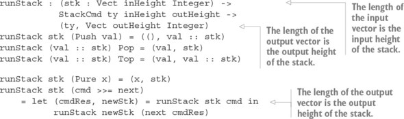
If you try runStack with testAdd, passing it an initial empty stack, you’ll see that it returns the sum of the two elements that you push, and that the final stack is empty:
*Stack> runStack [] testAdd (30, []) : (Integer, Vect 0 Integer)
You can also define functions like the following, which adds the top two elements on the stack, putting the result back onto the stack:
doAdd : StackCmd () (S (S height)) (S height) doAdd = do val1 <- Pop val2 <- Pop Push (val1 + val2)
The input state S (S height) means that the stack must have at least two elements on it, but, otherwise, it could be any height. If you try executing doAdd with an initial stack containing two elements, you’ll see that it results in a stack containing a single element that’s the sum of the two input elements:
*Stack> runStack [2,3] doAdd ((), [5]) : ((), Vect 1 Integer)
If the input state contains more than two elements, you’ll see that it results in a stack with a height one smaller than the input height. For example, an input stack of [2, 3, 4] results in an output stack with the value [2 + 3, 4]:
*Stack> runStack [2,3,4] doAdd ((), [5, 4]) : ((), Vect 2 Integer)You can add the two elements on the resulting stack with another call to doAdd:
*Stack> runStack [2,3,4] (do doAdd; doAdd) ((), [9]) : ((), Vect 1 Integer)
But trying one more doAdd would result in a type error, because there’s only one element left on the stack:
*Stack> runStack [2,3,4] (do doAdd; doAdd; doAdd) (input):1:34:When checking an application of constructor Main.>>=: Type mismatch between StackCmd () (S (S height)) (S height) (Type of doAdd) and StackCmd ty 1 outHeight (Expected type) Specifically: Type mismatch between S height and 0
This error means that you needed S (S height) elements on the stack (that is, at least two elements) but you only had S height (that is, at least one, but not necessarily any more). By putting the height of the stack in the type, therefore, you’ve explicitly specified the preconditions and postconditions on each operation, so you get a type error if you violate any of these.
13.2.3. Using a stack interactively: a stack-based calculator
If you add commands for reading from and writing to the console, you can write a console application for manipulating the stack and implement a stack-based calculator. A user can either enter a number, which pushes the number onto the stack, or add, which adds the top two stack items, pushes the result onto the stack, and displays the result. A typical session might go as follows:
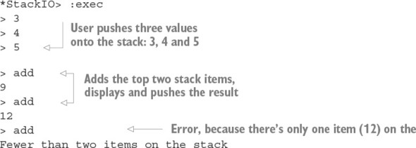
Figure 13.3 shows how each of the valid inputs in this session affects the contents of the stack. Every time the user enters an integer, the stack size grows by one, and every time the user enters add, the stack size decreases by one, as long as there are two items to add.
Figure 13.3. How each user input affects the contents of the stack
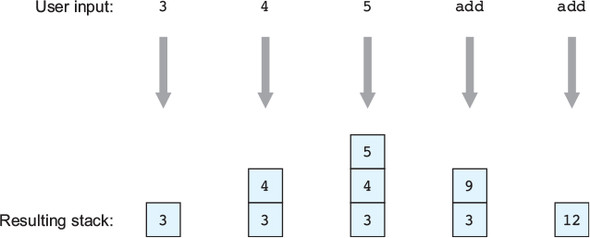
Listing 13.9. Extending StackCmd to support console I/O with the commands GetStr and PutStr (StackIO.idr)
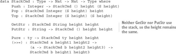
Dependent states in the Effects library
I mentioned the Effects library in chapter 12, which allows you to combine effects like state and console I/O without having to define a new type, like StackCmd here. The Effects library supports descriptions of state transitions and dependent state as in StackCmd. I won’t describe the Effects library further in this book, but learning about the principles of dependent state here will mean that you’ll be able to learn how to use the more flexible Effects library more readily.
You’ll also need to update runStack to support the two new commands. Because GetStr and PutStr describe interactive actions, you’ll need to update the type of runStack to return IO actions. Here’s the updated runStack.
Listing 13.10. Updating runStack to support the interactive commands GetStr and PutStr (StackIO.idr)
runStack : (stk : Vect inHeight Integer) -> StackCmd ty inHeight outHeight -> IO (ty, Vect outHeight Integer) runStack stk (Push val) = pure ((), val :: stk) runStack (val :: stk) Pop = pure (val, stk) runStack (val :: stk) Top = pure (val, val :: stk) runStack stk GetStr = do x <- getLine pure (x, stk) runStack stk (PutStr x) = do putStr x pure ((), stk) runStack stk (Pure x) = pure (x, stk) runStack stk (x >>= f) = do (x', newStk) <- runStack stk x runStack newStk (f x')
As with the vending machine, you’ll describe infinite sequences of StackCmd operations in total functions by defining a separate StackIO type for describing infinite streams of stack operations. The following listing shows how you can define StackIO and how to run StackIO sequences, given an initial state for the stack.
Listing 13.11. Defining infinite sequences of interactive stack operations (StackIO.idr)
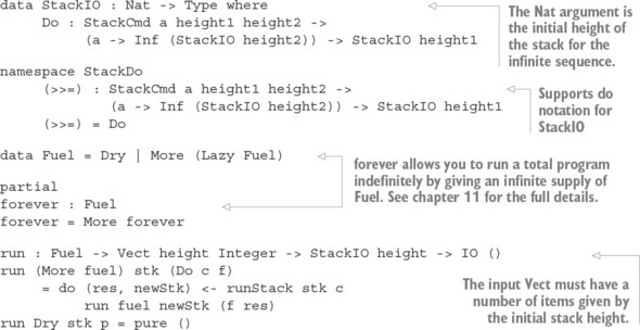
The interactive calculator follows a similar pattern to the implementation of the vending machine. The next listing shows an outline of the main loop, which reads an input, parses it into a command type, and processes the command if the input is valid.
Listing 13.12. Outline of an interactive stack-based calculator (StackIO.idr)
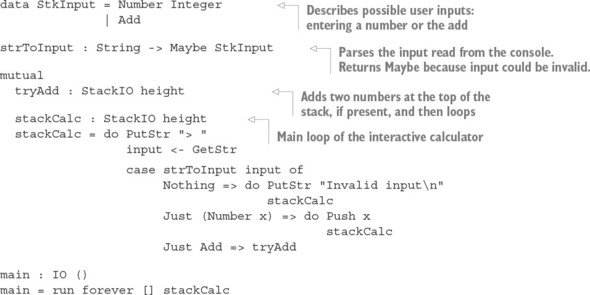
Listing 13.13. Reading user input for the stack-based calculator (StackIO.idr)
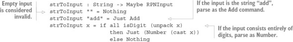
Finally, the next listing shows the definition of tryAdd. Like vend and refill in the vending machine implementation, you need to match on the initial state to make sure that there are enough items on the stack to add.
Listing 13.14. Adding the top two elements on the stack, if they’re present (StackIO.idr)
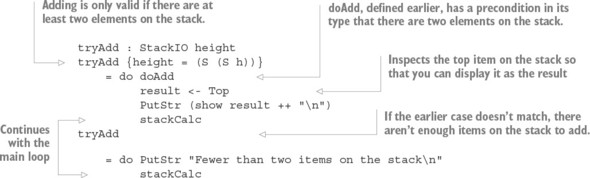
You can check that stackCalc is total at the REPL:
*StackIO> :total stackCalc Main.stackCalc is Total
By separating the looping component (StackIO) from the terminating component (StackCmd), and by giving precise types to the operations, you can be sure that stackCalc has at least the following properties, as long as it’s total:
- It will continue running indefinitely.
- It will never crash due to user input that isn’t handled.
- It will never crash due to a stack overflow.
Exercises
- Add user commands to the stack-based calculator for subtract and multiply. You can test these as follows:
*ex_13_2> :exec > 5 > 3 > subtract 2 > 8 > multiply 16
- Add a negate user command to the stack-based calculator for negating the top item on the stack. You can test this as follows:
> 10 > negate -10
- Add a discard user command that removes the top item from the stack. You can test this as follows:
> 3 > 4 > discard Discarded 4 > add Fewer than two items on the stack
- Add a duplicate user command that duplicates the top item on the stack. You can test this as follows:
> 2 > duplicate Duplicated 2 > add 4
13.3. Summary
- Data types can model state machines by using each data constructor to describe a state transition.
- You can describe how a command changes the state of a system by giving the input and output states of the system as part of the command’s type.
- Developing sequences of state transitions interactively, using holes, means you can check the required input and output states of a sequence of commands.
- Types can model infinite state spaces as well as finite states.
- Sequences of commands give verified sequences of state transitions because a sequence of commands will only type-check if it describes a valid sequence of state transitions.
- You can represent mutable dependently typed state by putting the arguments to the dependent type in the state transitions. For example, you can use the length of a vector to represent the height of a stack.
Chapter 14. Dependent state machines: handling feedback and errors
This chapter covers
- Handling errors in state transitions
- Developing protocol implementations interactively
- Guaranteeing security properties in types
As you saw in the previous chapter, you can describe the valid state transitions of a state machine in a dependent type, indexed by the required input state of an operation (its precondition) and the output state (its postcondition). By defining valid state transitions in the type, you can be sure that a program that type-checks is guaranteed to describe a valid sequence of state transitions.
You saw two examples, a description of a door and a simulation of a vending machine, and in each case we gave precise types to the operations to describe how they affected the state. But we didn’t consider the possibility that any of the operations could fail:
- What if, when you try to open the door, it’s jammed? What if, even though you’ve run the Open operation, it’s still in the DoorClosed state?
- What if, when you insert a coin in the vending machine, the machine rejects the coin?
In almost any realistic setting, when you try to give precise types to describe a state machine, you’ll need to consider the possibility of the operation failing, or of an unexpected response:
- Like the DoorState, you might represent the state of a file handle (open or closed) in a type, but if you try to open a file, the file might not exist or you might not have permission to open it.
- You might represent a secure communication protocol in a state machine, but whether you can progress in the protocol depends on receiving valid responses from the network to any request you send.
- You might represent the state of a bank’s automated teller machine (ATM) in a type (waiting for a card, waiting for PIN entry, and so on), but you can only move to a state where the machine can dispense cash if checking the user’s PIN is successful.
In these cases, you’re not in complete control of how the system state changes. You can request a change in the state (opening a file, sending a message, and so on) but whether and how the state changes in practice depends on the response you receive from the environment. In this chapter, you’ll see how to deal with the possibility of an operation failing by allowing a state transition to depend on the result of an operation.
You’ll also see how to deal with state changes that might depend on user input—we’ll look at the state transitions involved in modeling an ATM, where user input determines whether the machine can dispense cash. We’ll begin by revisiting the model of the door from chapter 13 and see how to deal with the possibility that the door might jam, so the Open operation fails.
14.1. Dealing with errors in state transitions
In the previous chapter, you defined a DoorCmd data type for modeling state transitions on a door, as illustrated by the state transition diagram in figure 14.1.
Figure 14.1. A state transition diagram showing the states and operations on a door
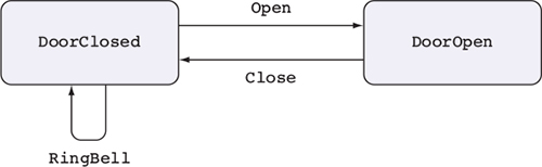
Listing 14.1 recaps the definition of DoorCmd, which models the state transition system in figure 14.1.
Listing 14.1. Modeling the door state machine in a type
data DoorState = DoorClosed | DoorOpen data DoorCmd : Type -> DoorState -> DoorState -> Type where Open : DoorCmd () DoorClosed DoorOpen Close : DoorCmd () DoorOpen DoorClosed RingBell : DoorCmd () DoorClosed DoorClosed Pure : ty -> DoorCmd ty state state (>>=) : DoorCmd a state1 state2 -> (a -> DoorCmd b state2 state3) -> DoorCmd b state1 state3In this model, you’re in complete control of how each operation moves from one state to another. For example, the type of Open states that it always starts with a door in the DoorClosed state, and it always ends with a door in the DoorOpen state:
Open : DoorCmd () DoorClosed DoorOpen
Reality is not always so accommodating, however! If you were to implement this with some real hardware, such as a sliding door operated by pressing a button, you’d need to consider the possibility of hardware problems such as the door jamming. In this section, we’ll refine the door model to capture this possibility of failure, and see how this affects the implementation of programs that follow the protocol.
14.1.1. Refining the door model: representing failure
Open could fail due to the door being jammed, so we need a way to represent whether it was successful. We could define an enumeration type to describe the possible results of opening the door:
data DoorResult = OK | Jammed
Then, instead of producing the unit value, Open could return a DoorResult. We might try the following type for Open:
Open : DoorCmd DoorResult DoorClosed DoorOpen
Unfortunately, this isn’t quite right because it still says that opening the door causes the door to be in the DoorOpen state, whatever happens. Somehow, we need to express that Open causes the door to be in either the DoorClosed or DoorOpen state, depending on the value of the DoorResult it produces. Figure 14.2 illustrates the state machine we’d like to implement.
Figure 14.2. A state transition diagram showing the states and operations on a door, where opening the door might fail
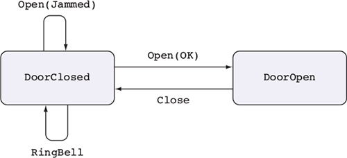
You can achieve this by changing the type of DoorCmd to allow the output state to be calculated from the return value. Figure 14.3 illustrates how you can refine the type of DoorCmd to achieve this.
Figure 14.3. New type for DoorCmd, where the output state of an operation is computed from the return value of the operation
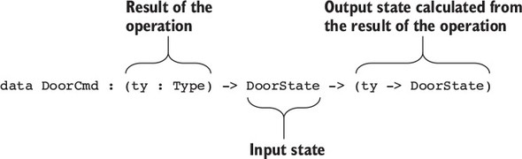
Here, you’ve given a name to the return type of the operation, ty, and said that the output state is computed by a function that takes a ty as an input. Now, when you define the type of Open (and indeed all of the DoorCmd operations), you give an expression for the output state, explaining how the output state is computed from the return value, of type DoorResult:
Open : DoorCmd DoorResult DoorClosed (\res => case res of OK => DoorOpen Jammed => DoorClosed)
This encodes exactly what the state transition diagram in figure 14.2 illustrates. That is, the output state of Open can be one of the following:
- DoorOpen—If Open returns OK
- DoorClosed—If Open returns Jammed
Although you won’t know the value of res until you run the operation, you can at least use the type to explain the possible states the door will be in given the result of Open. Listing 14.2 shows the complete DoorCmd type declaration after this refinement. It also adds Display, so you can display logging messages if necessary.
Listing 14.2. The refined DoorCmd type, allowing the output state of each operation to be computed from the return value of the operation (DoorJam.idr)
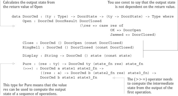
*DoorJam> :t const const : a -> b -> a
It ignores its second argument and returns its first. So, if you say const Door-Closed for the output state of an operation, that gives you a function that ignores the result of the function and always returns DoorClosed.
In the previous definition of DoorCmd, in listing 14.1, you used the (>>=) operator to explain that the output state of the first operation should be the input state of the second:
(>>=) : DoorCmd a state1 state2 -> (a -> DoorCmd b state2 state3) -> DoorCmd b state1 state3
It’s now slightly more complicated, because the return value of the first operation affects the input state of the second:
(>>=) : DoorCmd a state1 state2_fn -> ((res : a) -> DoorCmd b (state2_fn res) state3_fn) -> DoorCmd b state1 state3_fnThis works as follows:
- The first operation returns a value of type a, and the output state is computed from a state2_fn function once you know the result of the operation.
- When you come to the second operation, you’ll know the result of the first operation, named res, so it has an input state of state2_fn res.
- The combined operation has an input state of state1 (the input state of the first operation) and an output state computed from the result of the second operation, using state3_fn.
Defining DoorCmd this way gives you more precision in defining the state transitions, and it means that when you define functions using DoorCmd, the types of the operations require you to execute any necessary checks before continuing. For example, after you try to Open a door, you can’t execute any further door operations until you’ve checked the result. We’ll look at how this works by revisiting our earlier example, doorProg.
14.1.2. A verified, error-checking, door-protocol description
In chapter 13, you implemented a function using DoorCmd as a sequence of actions to ring the bell, and open and then close the door, and you used the types to verify that the sequence of actions was valid. You wrote doorProg as follows:
doorProg : DoorCmd () DoorClosed DoorClosed doorProg = do RingBell Open Close
Now that you’ve refined the type of DoorCmd so that the output state is computed from the result of the operation, you’ll need to write the type differently:
doorProg : DoorCmd () DoorClosed (const DoorClosed)
That is, the output state isn’t affected by the result, so you use const, which ignores its second argument and returns its first unchanged. But if you try implementing doorProg as before, without checking the result of Open, you’ll get an error:
doorProg : DoorCmd () DoorClosed (const DoorClosed) doorProg = do RingBell Open Close
The error happens when you try to use Close. Its type requires that the input state is DoorOpen, but in fact its input state is computed from the result of Open:
When checking an application of constructor Main.>>=: Type mismatch between DoorCmd () DoorOpen (const DoorClosed) (Type of Close) and DoorCmd () ((\res => case res of OK => DoorOpen Jammed => DoorClosed) _) (\value => DoorClosed) (Expected type)To see how to avoid this problem, you can develop doorProg interactively, beginning from the following point:
doorProg : DoorCmd () DoorClosed (const DoorClosed) doorProg = do RingBell Open ?doorProg_rhs
Debugging type errors using holes
If you get a type error that’s hard to understand on its own, it’s often a good idea to replace the offending part of the program with a hole (as we did by replacing Close with ?doorProg_rhs), to see what the expected type is, along with any local variables in scope.
- Type, refine—If you check the type of ?doorProg_rhs, you’ll see this:
-------------------------------------- doorProg_rhs : DoorCmd () (case _ of OK => DoorOpen Jammed => DoorClosed) (\value => DoorClosed)
The output state you see here arises from the definition of const in the Prelude, and it’s a function that ignores its argument value and returns DoorClosed. The input state you’re looking for is calculated from some value, _. This value is the result of Open, which you haven’t named. Let’s call it jam:doorProg : DoorCmd () DoorClosed (const DoorClosed) doorProg = do RingBell jam <- Open ?doorProg_rhs
- Type— You’ll now see that the input state of the next operation is calculated from the value of jam:
jam : DoorResult -------------------------------------- doorProg_rhs : DoorCmd () (case jam of OK => DoorOpen Jammed => DoorClosed) (\value => DoorClosed)
- Define, type—Because the input state depends on the value of jam, you can make progress by inspecting the value of jam:
doorProg : DoorCmd () DoorClosed (const DoorClosed) doorProg = do RingBell jam <- Open case jam of case_val => ?doorProg_rhs
You’ll now see that the input state depends on the value of case_val:case_val : DoorResult jam : DoorResult -------------------------------------- doorProg_rhs : DoorCmd () (case case_val of OK => DoorOpen Jammed => DoorClosed) (\value => DoorClosed)
- Define, type—If you case-split on case_val, you should see that each branch of the case has a different type, calculated from the specific value of case_val:
doorProg : DoorCmd () DoorClosed (const DoorClosed) doorProg = do RingBell jam <- Open case jam of OK => ?doorProg_rhs_1 Jammed => ?doorProg_rhs_2
In ?doorProg_rhs_1, for example, jam has the value OK, so the door must have successfully opened:jam : DoorResult -------------------------------------- doorProg_rhs_1 : DoorCmd () DoorOpen (\value => DoorClosed)
In ?doorProg_rhs_2, on the other hand, the door is jammed, so it’s still in the DoorClosed state:jam : DoorResult -------------------------------------- doorProg_rhs_2 : DoorCmd () DoorClosed (\value => DoorClosed)
- Refine— To complete the definition, you can display a log message in each case, and if the door is open, close it again:
doorProg : DoorCmd () DoorClosed (const DoorClosed) doorProg = do RingBell jam <- Open case jam of OK => do Display "Glad To Be Of Service" Close Jammed => Display "Door Jammed"
The type of Open means that you need to check the state of the door before you execute any further operations that need to know the door’s state. In particular, you can’t Close the door unless you’ve successfully opened it. You don’t have to check immediately, though. For example, you can display a message between opening the door and checking the result:
doorProg : DoorCmd () DoorClosed (const DoorClosed) doorProg = do RingBell jam <- Open Display "Trying to open the door" case jam of OK => do Display "Glad To Be Of Service" Close Jammed => Display "Door Jammed"
This is valid, because the precondition on Display doesn’t require the door to be in a specific state; any will do, and Display won’t change the state.
Using pattern-matching bindings, which you first saw in chapter 5, you can also define doorProg more concisely, as follows:
doorProg : DoorCmd () DoorClosed (const DoorClosed) doorProg = do RingBell OK <- Open | Jammed => Display "Door Jammed" Display "Glad To Be Of Service" Close
This gives a default path through the sequence of actions, when Open returns OK, and an alternative action when Open returns Jammed. Using pattern-matching bindings makes it easier to write longer sequences of actions, where some of the actions might fail. For example, you can open and close the door twice and abandon the sequence if either fails:
doorProg : DoorCmd () DoorClosed (const DoorClosed) doorProg = do RingBell OK <- Open | Jammed => Display "Door Jammed" Display "Glad To Be Of Service" Close OK <- Open | Jammed => Display "Door Jammed" Display "Glad To Be Of Service" Close
This example describes a protocol in the type, and it explicitly says where an operation might fail. In doorProg, the type of Open means that you need to check its result before you can proceed with any further operations that change the state.
The type of Pure in DoorCmd allows you to define functions like the following, where the call to Pure changes the state:
logOpen : DoorCmd DoorResult DoorClosed (\res => case res of OK => DoorOpen Jammed => DoorClosed) logOpen = do Display "Trying to open the door" OK <- Open | Jammed => do Display "Jammed" Pure Jammed Display "Success" Pure OKIf you replace the last line, Pure OK, with a hole, ?pure_ok, you’ll see that it has an input state of DoorOpen, and the output state (of the entire logOpen function) needs to be a function that computes its output state:
pure_ok : DoorCmd DoorResult DoorOpen (\res => case res of OK => DoorOpen Jammed => DoorClosed)
The type of Pure is designed to work in this situation:
Pure : (res : ty) -> DoorCmd ty (state_fn res) state_fn
Here, state_fn is the function containing the case block, and Pure must take OK as an argument to have the correct input state for ?pure_ok.
You now have a definition of DoorCmd that precisely describes the protocol for opening and closing doors, capturing the possibility of failure. But you haven’t yet seen how the corresponding run function works, which is where the result of an Open operation would be produced in practice. We’ll look at this next, in the context of a larger example: an ATM. We’ll also look at how state can change according to user input.
14.2. Security properties in types: modeling an ATM
You can use explicit states in the types of operations to guarantee, by type checking, that a system will only execute security-critical operations when it’s in a valid state to do so. For example, an ATM should only dispense cash when a user has inserted their card and entered a correct PIN. This is a typical sequence of operations on an ATM:
- A user inserts their bank card.
- The machine prompts the user for their PIN, to check that the user is entitled to use the card.
- If PIN entry is successful, the machine prompts the user for an amount of money, and then dispenses cash.
If the user enters the correct PIN, the machine will be in a state to dispense cash; otherwise, it won’t be. In this section, we’ll define a model for an ATM and see how to change the state of the machine, in its type, based on user input.
Security property of the ATM
In this model, we’ll omit some of the finer details of banking, such as accessing and updating the user’s bank account, and checking the PIN securely, which would be done with separate state machines. We’ll focus on one important security property we want to maintain: the machine must only dispense cash when there is a validated card in the machine.
As with the door model, we’ll begin by defining the possible states of the ATM and the operations that can change the ATM’s state. Once we know how the operations
affect the state, we can define a data type for representing the operations on the machine.14.2.1. Defining states for the ATM
An ATM is either waiting for a user to begin an interaction, waiting for the user to enter their PIN, or ready to dispense cash after validating a PIN. So an ATM, in our model, can be in one of the following states:
- Ready—The ATM is ready and waiting for a card to be inserted.
- CardInserted—There is a card inside the ATM, but the system has not yet checked a PIN entry against the card.
- Session—There is a card inside the ATM and the user has entered a valid PIN for the card, so a validated session is in progress.
We’ll validate the card by checking that the user inputs a correct PIN. In the vending machine in chapter 13, you also had to check that an input was valid, but in that case you could check the command locally. Here, we’ll assume that there’s an external service to check the PIN, so we won’t know until runtime which inputs will result in which states.
The machine supports the following basic operations, each of which may have preconditions and postconditions on the state of the machine:
- InsertCard—Waits for a user to insert a card
- EjectCard—Ejects a card from the machine, as long as there’s a card in the machine
- GetPIN—Reads a user’s PIN, as long as there’s a card in the machine
- CheckPIN—Checks whether an entered PIN is valid
- Dispense—Dispenses cash as long as there’s a validated card in the machine
- GetAmount—Reads from the user an amount to dispense
- Message—Displays a message to the user
Figure 14.4 illustrates how these operations affect the state of the machine.
Figure 14.4. A state machine describing the states and operations on an ATM. This omits operations (such as GetAmount) that are valid in all states.
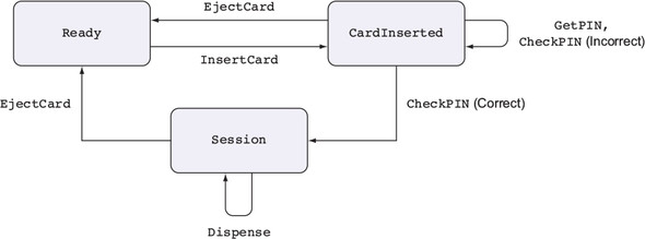
14.2.2. Defining a type for the ATM
Listing 14.3 defines an ATMCmd type that represents the state transitions of operations on an ATM in Idris code. It also includes GetAmount and Message, which are valid in all states and don’t affect the state, and the usual operations Pure and (>>=). The type of EjectCard is slightly simplified; we’ll refine this in section 14.2.4.
Listing 14.3. A type for representing the commands of an ATM, and how they affect the ATM’s state (ATM.idr)
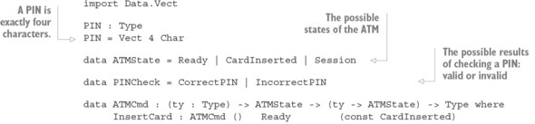
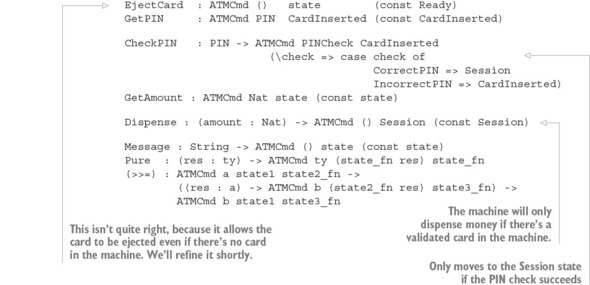
Using ATMCmd, you can write a function that describes a session on an ATM, from the user inserting a card to the machine dispensing cash. Listing 14.4 shows the beginning of an atm function that waits for a user to insert a card, prompts for a PIN, and then checks the result. I’ve left a hole for the rest of the sequence, in which we’ll check the PIN and dispense cash if the PIN is valid.
Listing 14.4. An atm function describing a sequence of operations on an ATM (ATM.idr)
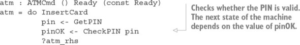
You can complete atm as follows:
- Type, define—If you check the type of the ?atm_rhs hole, you’ll see that you begin in a state that depends on the value of pinOK, and you need to end in the Ready state:
pin : Vect 4 Char pinOK : PINCheck -------------------------------------- atm_rhs : ATMCmd () (case pinOK of CorrectPIN => Session IncorrectPIN => CardInserted) (\value => Ready)
The type here suggests you can proceed by checking the value of pinOK:atm : ATMCmd () Ready (const Ready) atm = do InsertCard pin <- GetPIN pinOK <- CheckPIN pin case pinOK of CorrectPIN => ?atm_rhs_1 IncorrectPIN => ?atm_rhs_2
- Type— If you check ?atm_rhs_1 and ?atm_rhs_2, you’ll see that the state is different in each case. In ?atm_rhs_1, the PIN was found to be valid, so you have a validated session:
pinOK : PINCheck pin : Vect 4 Char -------------------------------------- atm_rhs_1 : ATMCmd () Session (\value => Ready)
In ?atm_rhs_2, on the other hand, the PIN was found to be invalid, so you’re still in the CardInserted state:pinOK : PINCheck pin : Vect 4 Char -------------------------------------- atm_rhs_2 : ATMCmd () CardInserted (\value => Ready)
- Refine— In ?atm_rhs_1, you can now dispense cash, so you can prompt for an amount and dispense that:
case pinOK of CorrectPIN => do cash <- GetAmount Dispense cash ?atm_rhs_1 IncorrectPIN => ?atm_rhs_2
- Type, refine—The input state of ?atm_rhs_1 is still Session, so before you finish you need to get back to the Ready state:
pin : Vect 4 Char pinOK : PINCheck cash : Nat -------------------------------------- atm_rhs_1 : ATMCmd () Session (\value => Ready)
You can achieve this by ejecting the card:case pinOK of CorrectPIN => do cash <- GetAmount Dispense cash EjectCard IncorrectPIN => ?atm_rhs_2
- Refine— For ?atm_rhs_2, the PIN was invalid, so the simplest thing to do is eject the card, leading to the following completed definition:
atm : ATMCmd () Ready (const Ready) atm = do InsertCard pin <- GetPIN pinOK <- CheckPIN pin case pinOK of CorrectPIN => do cash <- GetAmount Dispense cash EjectCard IncorrectPIN => EjectCard
There are other ways you could define atm. For example, it would be helpful to display messages to the user. Also, in practice, ATMs typically don’t check the PIN until just before dispensing cash. The next listing shows this alternative way of implementing atm.
Listing 14.5. An alternative implementation of atm, including messages to the user and checking the PIN later (ATM.idr)

14.2.3. Simulating an ATM at the console: executing ATMCmd
To try the atm function, you can write a console simulation of an ATM that produces IO actions for an ATMCmd description:
runATM : ATMCmd res inState outState_fn -> IO res
Given a sequence of ATMCmd that produces a result of type res, begins in state inState, and computes the result state with outState_fn, runATM gives a sequence of IO actions that produces a result, res. Let’s hardcode a single valid PIN for this simulation:
testPIN : Vect 4 Char testPIN = ['1', '2', '3', '4']
The following listing shows a console simulation of an ATM that uses this hardcoded PIN. In this simulation, many of the commands prompt for an input on the console and return the value read.
Listing 14.6. A console simulation of an ATM (ATM.idr)
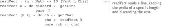
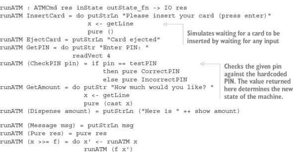
14.2.4. Refining preconditions using auto-implicits
One feature of the state machine in figure 14.4 that ATMCmd type doesn’t quite capture is that ejecting the card should only be allowed when there’s a card in the machine. Instead, you have the following type:
EjectCard : ATMCmd () state (const Ready)
That is, you can try to eject a card in any input state, even when there’s no card in the machine. But there are only two states when it’s okay to eject a card: CardInserted and Session. You shouldn’t be able to write the following function, because the machine is ejecting a card in the Ready state:
badATM : ATMCmd () Ready (const Ready) badATM = EjectCard
Somehow, you need both of the following types to work for EjectCard:
EjectCard : ATMCmd () CardInserted (const Ready) EjectCard : ATMCmd () Session (const Ready)
A data constructor like EjectCard can’t have two different types. You can, however, define a predicate on ATMState that will allow you to restrict the possible input states of EjectCard to those that are valid. We discussed predicates in chapter 9, and you can define a HasCard predicate that describes the states in which a machine contains a card:
data HasCard : ATMState -> Type where HasCI : HasCard CardInserted HasSession : HasCard Session
You can only construct a value of type HasCard state when state is one of Card-Inserted or Session, so you can refine the type of EjectCard as follows:
EjectCard : HasCard state -> ATMCmd () state (const Ready)
If you do this, you’ll need to give values of type HasCard explicitly when using EjectCard. For example:
insertEject : ATMCmd () Ready (const Ready) insertEject = do InsertCard EjectCard HasCI
Having to write explicit values for the predicate will get tedious very quickly. Instead, you can use an auto implicit for the predicate, which you also saw in chapter 9:
EjectCard : {auto prf : HasCard state} -> ATMCmd () state (const Ready) Now, you can use EjectCard as before, and let Idris find the correct value for the predicate by searching through the possible data constructors for HasCard to see if any of them are valid:
insertEject : ATMCmd () Ready (const Ready) insertEject = do InsertCard EjectCard
For badATM, Idris shouldn’t be able to find a suitable value:
badATM : ATMCmd () Ready (const Ready) badATM = EjectCard
In this case, Idris will report an error, saying that it needs to find a value of type HasCard Ready for the predicate to EjectCard, but it can’t find one:
When checking argument prf to constructor Main.EjectCard: Can't find a value of type HasCard Ready
All of your other previous definitions, including the two versions of atm and the execution function runATM, will work without any alteration using this refined version of EjectCard.
Exercises
- The following type outlines a security system in which a user can log in with a password and then read a secret message, although there are some gaps:
data Access = LoggedOut | LoggedIn data PwdCheck = Correct | Incorrect data ShellCmd : (ty : Type) -> Access -> (ty -> Access) -> Type where Password : String -> ShellCmd PwdCheck ?password_in ?password_out Logout : ShellCmd () ?logout_in ?logout_out GetSecret : ShellCmd String ?getsecret_in ?getsecret_out PutStr : String -> ShellCmd () state (const state) Pure : (res : ty) -> ShellCmd ty (state_fn res) state_fn (>>=) : ShellCmd a state1 state2_fn -> ((res : a) -> ShellCmd b (state2_fn res) state3_fn) -> ShellCmd b state1 state3_fn
Fill in the holes in the following types:- Password—Reads a password and changes the state to LoggedIn or LoggedOut, depending on whether the password was correct
- Logout—Changes the state from LoggedIn to LoggedOut
- GetSecret—Reads a secret message as long as the state is LoggedIn
session : ShellCmd () LoggedOut (const LoggedOut) session = do Correct <- Password "wurzel" | Incorrect => PutStr "Wrong password" msg <- GetSecret PutStr ("Secret code: " ++ show msg ++ "\n") LogoutThe following functions should not type-check:sessionBad : ShellCmd () LoggedOut (const LoggedOut) sessionBad = do Password "wurzel" msg <- GetSecret PutStr ("Secret code: " ++ show msg ++ "\n") Logout noLogout : ShellCmd () LoggedOut (const LoggedOut) noLogout = do Correct <- Password "wurzel" | Incorrect => PutStr "Wrong password" msg <- GetSecret PutStr ("Secret code: " ++ show msg ++ "\n") - When inserting a coin into the vending machine defined in chapter 13, the machine could reject the coin. You can represent this by changing the types of MachineCmd and InsertCoin. An operation in MachineCmd can change the state based on its result:
data MachineCmd : (ty : Type) -> VendState -> (ty -> VendState) -> Type
Then, InsertCoin can return whether or not the coin insertion was successful and change the state accordingly:InsertCoin : MachineCmd CoinResult (pounds, chocs) (\res => case res of Inserted => (S pounds, chocs) Rejected => (pounds, chocs))
Define the CoinResult type, and then make this change to MachineCmd in Vending .idr. Also, refine the types of the other commands and the implementation of machineLoop as necessary.
14.3. A verified guessing game: describing rules in types
As a concluding example in this chapter, we’ll look at how you can use a type to represent the rules of a game precisely, and be sure that any implementation of the game follows the rules correctly. We’ll revisit an example from chapter 9, the word-guessing game Hangman.
To recap how this worked, you defined a WordState type to represent the state of the game. WordState was defined as follows, including the number of guesses and letters remaining as arguments:
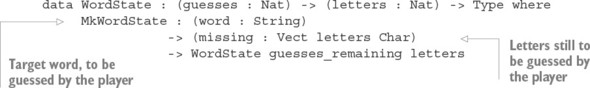
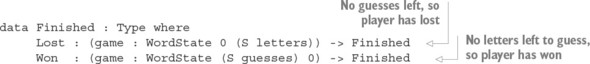
Given these, you defined a main loop called game, which took a WordState with both guesses and letters remaining, and looped until the game was complete:
game : WordState (S guesses) (S letters) -> IO Finished
In the implementation, you used the type to help direct you to a working implementation. But you could also have written an incorrect implementation of the game using this type. For example, the following implementation of game would also be well typed, but wrong, because it returns a losing game state in all cases:
game : WordState (S guesses) (S letters) -> IO Finished game state = pure (Lost (MkWordState "ANYTHING" ['A']))
Although the type allows you to express the game state precisely and helps you give types to intermediate operations (such as processing a guess), it doesn’t guarantee that the implementation follows the rules of the game correctly. In the preceding implementation, it’s impossible for the player to win!
In this section, instead of defining a WordState type and then trusting that game will follow the rules of the game correctly, we’ll define the rules of the game precisely in a state type. Just as DoorCmd expresses when we can execute operations on a door, and ATMCmd expresses when we can execute operations on an ATM, we can define a dependent GameCmd type that expresses when it’s valid to execute particular operations in a game, and what the effect on those operations will be. As with the door and ATM examples, we’ll begin by defining the states and the operations that can be executed on those states.
14.3.1. Defining an abstract game state and operations
First, we’ll think about how we can define the rules of the game in abstract terms, without worrying about the details of the implementation. A game can be in one of the following states:
- NotRunning—There is no game currently in progress. Either the game hasn’t started and there’s no word yet to guess, or the game is complete.
- Running—There is a game in progress, and the player has a number of guesses remaining and letters still to guess.
In the case of Running, we’ll annotate the state with the number of guesses and letters remaining, just as we did with WordState earlier, because this means we’ll be able to
describe precisely when a game has been won (no letters to guess) or lost (no guesses remaining). We can express the possible states in the following data type:data GameState : Type where NotRunning : GameState Running : (guesses : Nat) -> (letters : Nat) -> GameState
Then, we’ll support some basic operations for manipulating the game state:
- NewGame—Initializes a game with a word for the player to guess
- Guess—Allows the player to guess a letter
- Won—Declares that the player has won the game
- Lost—Declares that the player has lost the game
Figure 14.5 illustrates how these basic operations affect the game state. There are additional preconditions on Won and Lost: we can only declare that the player has won the game if there are no letters left to guess, and we can only declare that the player has lost if there are no guesses remaining.
Figure 14.5. State transition diagram for Hangman. The Running state also holds the number of letters and guesses remaining. Won requires the number of letters to be zero, and Lost requires the number of guesses to be zero.
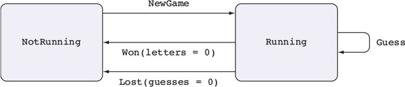
The next step is to represent these state transitions precisely in a dependent type, including the specific rules about the number of guesses and letters required for each operation to be valid.
14.3.2. Defining a type for the game state
We’ll define a GameCmd type that describes the possible operations you can run that affect GameState.
The next listing shows the types of NewGame, Won, and Lost from figure 14.5. As usual, Pure and (>>=) are included so that you can introduce pure values and sequence operations.
Listing 14.7. Beginning to define GameCmd (Hangman.idr)
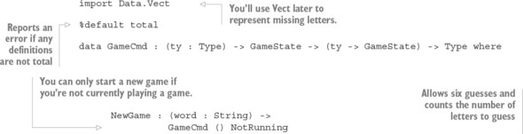
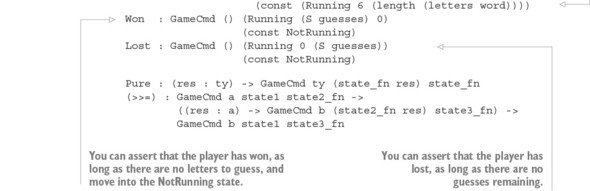
You can get the different letters in a word using letters, which converts the word to uppercase, then converts it to a List Char, and finally removes any duplicate elements:

Listing 14.8 adds a Guess operation to GameCmd. The type of Guess has a precondition and a postcondition that explain how the guess affects the game:
- As a precondition, there must be at least one guess available (S guesses) and at least one letter still to guess (S letters), or attempting to guess a letter won’t type-check.
- As a postcondition, the number of guesses will reduce if the guess was incorrect, and the number of letters will reduce if the guess was correct.
Listing 14.8. Adding a Guess operation (Hangman.idr)
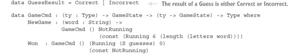
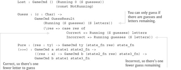
data GameCmd : (ty : Type) -> GameState -> (ty -> GameState) -> Type where {- Continued from Listing 14.8 -} ShowState : GameCmd () state (const state) Message : String -> GameCmd () state (const state) ReadGuess : GameCmd Char state (const state) Displaying the game state should display the known letters in the target word and the number of guesses remaining. For example, if the target word is TESTING and you’ve already guessed T, with six guesses remaining, ShowState should display the following:
T--T--- 6 guesses left
When you actually implement the game, it’s useful to support indefinitely long game loops. For example, once you finish a game, a player might want to start a new game. The next listing defines a GameLoop type, using Inf to note that execution might continue indefinitely.
Listing 14.9. A type for describing potentially infinite game loops (Hangman.idr)
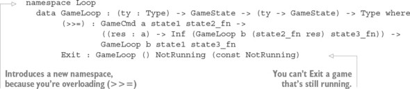
You can use the operations in GameLoop and GameCmd to define the following function, which implements a game loop:
gameLoop : GameLoop () (Running (S guesses) (S letters)) (const NotRunning)
Once you have a well-typed, total implementation of gameLoop, you’ll know that it’s a valid implementation of the rules. Neither the game nor the player will be able to
cheat by breaking the rules as they’re defined in GameCmd. You can only call gameLoop on a properly initialized game, with a word to guess, and any implementation must be a complete implementation of the game because the only way to finish a GameLoop is by calling Exit, which requires a game to be in the NotRunning state.14.3.3. Implementing the game
We’ll implement gameLoop interactively and see how the state of the game progresses by checking types as we go.
To begin, you can create a skeleton definition, bringing guesses and letters from the type into scope, because you’ll need to inspect them to check the player’s progress later:
gameLoop : GameLoop () (Running (S guesses) (S letters)) (const NotRunning) gameLoop {guesses} {letters} = ?gameLoop_rhs To implement gameLoop, take the following steps:
- Refine— At the start of each iteration of gameLoop, you’ll display the current state of the game using ShowState, read a guess from the user, and then check whether it was correct:
gameLoop : GameLoop () (Running (S guesses) (S letters)) (const NotRunning) gameLoop {guesses} {letters} = do ShowState g <- ReadGuess ok <- Guess g ?gameLoop_rhs - Type, define—If you check the type of ?gameLoop_rhs now, you’ll see that the current state of the game depends on whether the guess was correct or not:
letters : Nat guesses : Nat g : Char ok : GuessResult -------------------------------------- gameLoop_rhs : GameLoop () (case ok of Correct => Running (S guesses) letters Incorrect => Running guesses (S letters)) (\value => NotRunning)
To make progress, you’ll need to inspect ok to establish which state the game is in:gameLoop : GameLoop () (Running (S guesses) (S letters)) (const NotRunning) gameLoop {guesses} {letters} = do ShowState g <- ReadGuess ok <- Guess g case ok of Correct => ?gameLoop_rhs_1 Incorrect => ?gameLoop_rhs_2 - Type, define—In ?gameLoop_rhs_1, the guess was correct, so the number of letters remaining is reduced, as you can see by checking its type:
ok : GuessResult letters : Nat guesses : Nat g : Char -------------------------------------- gameLoop_rhs_1 : GameLoop () (Running (S guesses) letters) (\value => NotRunning)
You can only continue with gameLoop if there are both letters and guesses remaining, because its input state is Running (S guesses) (S letters). To decide how to continue, you’ll need to check the current value of letters:case ok of Correct => case letters of Z => ?gameLoop_rhs_3 S k => ?gameLoop_rhs_4 Incorrect => ?gameLoop_rhs_2
- Refine— In ?gameLoop_rhs_3, there are no letters left to guess, so the player has won. You can declare that the player has won with Won, moving to the Not-Running state. Then display the final state and exit:
case ok of Correct => case letters of Z => do Won ShowState Exit S k => ?gameLoop_rhs_4 Incorrect => ?gameLoop_rhs_2
You need to Exit explicitly, because Exit is the only way to break out of a GameLoop. You can only Exit a game in the NotRunning state. - Refine— In ?gameLoop_rhs_4, there are still letters to guess, so you can display a message and continue with gameLoop:
case ok of Correct => case letters of Z => do Won ShowState Exit S k => do Message "Correct" gameLoop Incorrect => ?gameLoop_rhs_2
The Incorrect case works similarly, checking whether guesses are still available and declaring that the player has lost if not. The following listing gives the complete definition, for reference.
Listing 14.10. A complete implementation of gameLoop (Hangman.idr)
gameLoop : GameLoop () (Running (S guesses) (S letters)) (const NotRunning) gameLoop {guesses} {letters} = do ShowState g <- ReadGuess ok <- Guess g case ok of Correct => case letters of Z => do Won ShowState Exit S k => do Message "Correct" gameLoop Incorrect => case guesses of Z => do Lost ShowState Exit (S k) => do Message "Incorrect" gameLoop You’ll also need to initialize the game. For example, you could write a function to set up a new game, and then initiate the gameLoop: hangman : GameLoop () NotRunning (const NotRunning) hangman = do NewGame "testing" gameLoop
So far, you’ve only defined a data type that describes the actions in the game. The gameLoop function describes sequences of actions in a valid game of Hangman that follows the rules. In order to run the game, you’ll need to define a concrete representation of the game state and a function that translates a GameLoop to a sequence of IO actions.
14.3.4. Defining a concrete game state
In the stack example in chapter 13, we had an abstract state of the stack (the number of items on the stack), and a concrete state represented by a Vect of an appropriate length. Similarly, GameState is the abstract state of a game, describing only whether a game is running, and if so, how many guesses and letters are remaining.
In order to run a game, you’ll need to define a corresponding concrete game state that includes the specific target word and which specific letters are still to be guessed. The following listing defines a Game type with a GameState argument, representing the concrete data associated with an abstract game state.
Listing 14.11. Representing the concrete game state (Hangman.idr)
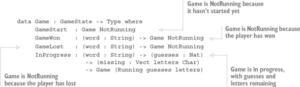
It’s convenient to define a Show implementation for Game so that you can easily display a string representation of a game’s progress.
Listing 14.12. A Show implementation for Game (Hangman.idr)
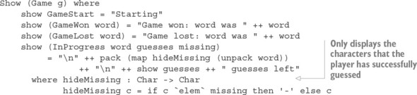
You can use Game to keep track of the concrete game state. When you execute a GameLoop, you’ll take a concrete game state as input, and return a result along with the updated game state:
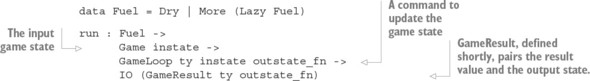
You use Fuel, because run potentially loops. In particular, when you read a Guess from the player, the only valid input is a single alphabetical character, so you’ll need to keep asking for input until it’s valid.
If you run out of fuel, the GameResult needs to say that execution failed. Otherwise, it needs to store the result of the operation and the new state. Crucially, the type of the new state might depend on the result; for example, the number of guesses available is different depending on whether Guess returns Correct or Incorrect. A GameResult, therefore, is one of the following:
- A pair of the result produced by executing the game and the output state, with a type calculated from the result
- An error, if run ran out of fuel
You can define GameResult as follows:
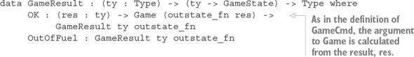
Now that you have a data type to represent the concrete state of a game—which takes the abstract state as an argument—along with a representation of the result, you’re ready to implement run.
14.3.5. Running the game: executing GameLoop
The next listing outlines the definition of run for GameLoop. This uses another function, runCmd, to execute GameCmd. There’s a hole for the definition of runCmd for the moment.
Listing 14.13. Running the game loop (Hangman.idr)
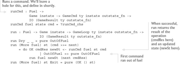
In run, when it’s successful, you use pure to return a pair of the result and the new state. Because you’ll often return a result in this form when executing a command, you can define a helper function, ok, to make this more concise:
ok : (res : ty) -> Game (outstate_fn res) -> IO (GameResult ty outstate_fn) ok res st = pure (OK res st)
Using ok, you can refine the last clause of run to the following:
run (More fuel) st Exit = ok () st
Listing 14.14 gives an outline definition of runCmd, leaving holes for the Guess and ReadGuess cases. In the other cases, you use ok to update the state as required by the type and execute IO actions as necessary.
Listing 14.14. Outline definition of runCmd (Hangman.idr)
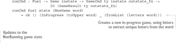
When a game is in progress, the game state uses the InProgress constructor of Game, which has the following type:
*Hangman> :t InProgress InProgress : String -> (guesses : Nat) -> Vect letters Char -> Game (Running guesses letters)
The third argument is a vector of the letters that are still to be guessed. So, in the Guess case, you check whether the guessed character is in the vector of missing letters:
You defined removeElem interactively in chapter 9 in the earlier implementation of Hangman. For convenience, I’ll repeat it here:
removeElem : (value : a) -> (xs : Vect (S n) a) -> {auto prf : Elem value xs} -> Vect n a removeElem value (value :: ys) {prf = Here} = ys removeElem {n = Z} value (y :: []) {prf = There later} = absurd later removeElem {n = (S k)} value (y :: ys) {prf = There later} = y :: removeElem value ys Finally, you need to define the ReadGuess case, which reads a character from the player. The input is only valid if it’s an alphabetical character, so you loop until the player enters a valid input:
This case might loop indefinitely if the user continues to enter invalid input, so runCmd takes Fuel as an argument and consumes fuel whenever there’s an invalid input. As a result, runCmd itself remains total because it either consumes fuel or processes a command on each recursive call. It’s important for runCmd to be total, because it means you know that executing a GameCmd will continue to make progress as long as there are commands to execute.
You’re now in a position to write the main program, using forever to ensure that, in practice, run never runs out of fuel. Add the following to the end of Hangman.idr:
You should now be able to execute the game at the REPL. Here’s an example:
*Hangman> :exec ------- 6 guesses left Guess: t Correct T--T--- 6 guesses left Guess: x Incorrect T--T--- 5 guesses left Guess: g Correct T--T--G 5 guesses left Guess: bad Invalid input Guess:
In this example, we’ve separated the description of the rules, in GameCmd and GameLoop, from the execution of the rules, in runCmd and run. Essentially, GameCmd and GameLoop define an interface for constructing a valid game of Hangman, correctly following the rules. Any well-typed total function using these types must be a correct implementation of the rules, or it wouldn’t have type-checked!
14.4. Summary
- You can get feedback from the environment by using the result of an operation to compute the output state of a command.
- A system might be in a different state after running a command, depending on whether the command was successful.
- Defining preconditions on operations allows you to express security properties in types, such as when it’s valid for an ATM to dispense cash.
- A system might change state according to whether a user’s input is valid in the current environment, such as whether a PIN or password is correct.
- Predicates and auto implicits help you describe valid input states of operations precisely.
- You can describe the rules of a game precisely in a type, so that a function that type-checks must be a valid implementation of the rules.
- You use an abstract state type to describe what operations do, and a concrete state, depending on the abstract state, to describe their corresponding implementations.
Chapter 15. Type-safe concurrent programming
This chapter covers
- Using concurrency primitives
- Defining a type for describing concurrent processes
- Using types to ensure concurrent processes communicate consistently
In Idris, a value of type IO () describes a sequence of actions for interacting with the user and operating system, which the runtime system executes sequentially. That is, it only executes one action at a time. You can refer to a sequence of interactive actions as a process.
As well as executing actions in sequence in a single process, it’s often useful to be able to execute multiple processes at the same time, concurrently, and to allow those processes to communicate with each other. In this chapter, I’ll introduce concurrent programming in Idris.
Message passing
Concurrent programming is a large topic, and there are several approaches to it that would fill books of their own. We’ll look at some small examples of message-passing concurrency, where processes
interact by sending messages to each other. Message passing is supported as a primitive by the Idris runtime system. In effect, sending a message to a process and receiving a reply corresponds to calling a method that returns a result in an object-oriented language.Concurrent programming has several advantages:
- You can continue to interact with a user while a large computation runs. For example, a user can continue browsing a web page while a large file downloads.
- You can display feedback on the progress of a large computation running in another process, such as displaying a progress bar for a download.
- You can take full advantage of the processing power of modern CPUs, dividing work between multiple processes running on separate CPU cores.
This chapter presents a larger example of type-driven development. First, I’ll introduce the primitives for concurrent programming in Idris, and describe the problems that can arise in concurrent processes in general. Then, I’ll present an initial attempt at a type for describing concurrent processes. This initial attempt will have some shortcomings, so we’ll refine it and arrive at a type that allows processes to communicate with each other safely and consistently.
15.1. Primitives for concurrent programming in Idris
The Idris base library provides a module, System.Concurrency.Channels, that contains primitives for starting concurrent processes and for allowing those processes to communicate with each other. This allows you, in theory, to write applications that make efficient use of your CPUs and that remain responsive even when executing complex calculations.
But despite its advantages, concurrent programming is notoriously error-prone. The need for multiple processes to interact with each other greatly increases a program’s complexity. For example, if you’re displaying a progress bar while a file downloads, the process downloading the file needs to coordinate with the process displaying the progress bar so that it knows how much of the file is downloaded. This complexity leads to new ways in which programs can fail at runtime:
- Deadlock— Two or more processes are waiting for each other to perform some action before they can continue.
- Race conditions— The behavior of a system depends on the ordering of actions in multiple concurrent processes.
The effect of a deadlock is that the processes concerned freeze, no longer accepting input or giving output. Two concurrent processes—let’s call them client and server—could deadlock if client is waiting to receive a message from server at the same time that server is waiting to receive a message from client. If this happens, both client and server will freeze.
Race conditions can be harder to identify. The pseudocode in figure 15.1 for client and server illustrates a race condition, where the value of the shared variable var depends on the order in which the concurrent operations execute. We’ll assume that the Read and Write operations respectively read and write the value of a shared mutable variable, so Read var reads the value of the shared variable var.Figure 15.1. Pseudocode for client and server, in which each process reads and writes a shared variable, var. This could lead to an unexpected result if lines A and C are executed before lines C and D.
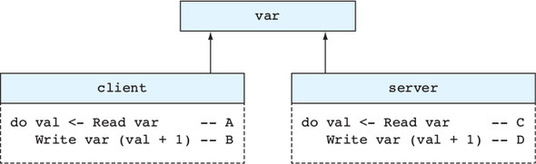
Here, client and server execute concurrently, and the final value of var depends on the order in which the operations A, B, C, and D are executed. A will always run before B, and C before D, but otherwise there are six possible orderings for the operations. Table 15.1 lists these orderings and the resulting value of var in each case, assuming an initial value of 1.
Table 15.1. Value of var for each sequence of operations in figure 15.1, given an initial value of 1 for var
| Operation order | Value of var |
|---|---|
| A, B, C, D | 3 |
| A, C, B, D | 2 |
| A, C, D, B | 2 |
| C, A, B, D | 2 |
| C, A, D, B | 2 |
| C, D, A, B | 3 |
As the table shows, with an initial value for var of 1, there are two possible results for var, depending on the order in which the Read and Write operations run. Here, there are only two processes with two operations each. As programs grow, the likelihood of this kind of nondeterministic result becomes much larger.
Later in this chapter, using a variety of techniques that we’ve discussed earlier in this book, you’ll see how to write concurrent programs in Idris, avoiding problems such as deadlock and race conditions. But first, you need to understand the primitives
that the Idris base library provides for concurrent programming and see the kinds of problems you’ll encounter when writing processes that need to coordinate with each other.15.1.1. Defining concurrent processes
In a complete Idris program, the main function, which has type IO (), describes the actions that the runtime system will execute when the program is run. The main function, therefore, describes the actions that are executed in a single process.
The actions we’ve used have described console and file I/O operations, but the runtime system also supports actions for starting new processes and sending messages between processes. There are primitive operations for the following actions:
- Creating a new process. Each process is associated with a unique process identifier (PID).
- Sending a message to a process identified by its PID.
- Receiving a message from another process.
Figure 15.2 illustrates one way we can use message passing to write concurrent processes that communicate with each other. In this figure, main and adder are two Idris processes, running concurrently, where each can send a message to the other.
Figure 15.2. Message-passing between processes. A main process sends an Add 2 3 message to an adder process, which replies by sending a 5 message back to main.
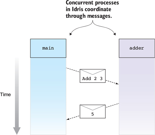
The message that main sends to adder uses the following type:
data Message = Add Nat Nat
In this example, after main sends the message Add 2 3 to the adder process, it expects to receive a reply with the result of adding 2 and 3. In this way, you can use concurrently running processes to implement services that respond to requests sent by other processes. Here, we have a service that performs addition, running in a separate process.
I’ll use this as a running example of concurrent processes. Next, you’ll see how to use the concurrency primitives that Idris provides to implement an adder service in a separate process, and how to use that service from main.15.1.2. The Channels library: primitive message passing
The System.Concurrency.Channels module, in the base library, defines data types and actions that allow Idris processes to create new processes and communicate with each other. It defines the following types:
- PID—Represents a process identifier. Every process is associated with a PID that allows you to set up a communication channel with the process.
- Channel—A link between two processes. It defines a communication channel along which you can send messages.
The System.Concurrency.Channels module also defines the following functions for creating new processes and setting up communication channels:
- spawn—Creates a new process for executing a sequence of actions of type IO (), and if successful returns its PID.
- connect—Initiates a communication channel to a running process.
- listen—Waits for another process to initiate a communication. When another process connects, it sets up a communication channel with that process.
Finally, the module defines operations for sending and receiving messages on a Channel. We’ll come to the type definitions in System.Concurrency.Channels shortly, but first let’s look at how the processes and channels are set up for the main and adder processes. The main process works as follows:
- Starts the adder process using spawn
- Sets up a communication channel to adder using connect
- Sends an Add 2 3 message on the channel
- Receives a reply on the channel with the result
Correspondingly, the adder process works as follows:
- Waits for another process to initiate a communication using listen and sets up a new communication channel when another process connects
- Receives a message on the channel containing the numbers to be added
- Sends a message on the channel with the result
- Returns to step 1, waiting for the next request
The adder process provides a long-running service that waits for incoming requests and sends replies to those requests. Once main has started the adder process, any other process can also send requests to adder, as long as it knows adder’s PID.
The first listing shows the type declarations for channels and PIDs in System.Concurrency.Channels and the functions you can use to create processes and set up communication channels.
Listing 15.1. Channels and PIDs (defined in System.Concurrency.Channels)
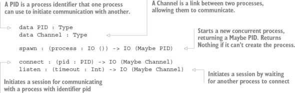
You can use spawn, listen, and connect to set up adder and main as separate processes. The following listing outlines a program that sets up the processes, leaving holes for the parts of the processes that send messages to each other.
Listing 15.2. Outline of a program that sets up an adder process (AdderChannel.idr)
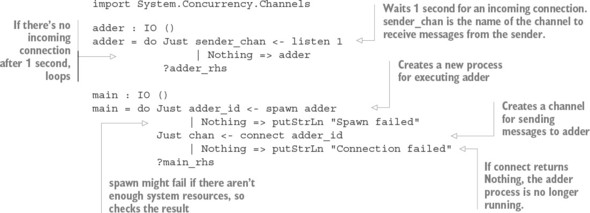
Now that you’ve set up the processes and channels, main can send a message to adder, and adder can reply. You can use the following primitives:
- unsafeSend—Sends a message of any type
- unsafeRecv—Receives a message of an expected type
As the names imply, these primitives are unsafe, because they don’t provide a way of checking that the sender and receiver are expecting messages to be sent in a specific order, or that they’re sending and receiving messages of consistent types. Nevertheless, for the moment we’ll use them to complete the implementations of main and adder. Later, in section 15.2, you’ll see how to make safe versions that ensure that processes send and receive messages with a consistent protocol.
Why support an unsafe Channel type?
It might seem surprising that Idris, a language that’s designed to support type-driven development, supports such unsafe concurrency primitives rather than something more sophisticated. The reason is that there are many possible methods for implementing safe concurrent programs in a type-driven way, and by providing unsafe underlying primitives, Idris is not limited to only one of them. You’ll see one such method shortly.
The following listing shows the type declarations for these primitive operations, defined in System.Concurrency.Channels.
Listing 15.3. Primitive message passing (defined in System.Concurrency.Channels)
unsafeSend : Channel -> (val : a) -> IO Bool unsafeRecv : (expected : Type) -> Channel -> IO (Maybe expected)
In the next listing, you can complete the definition of adder by receiving a request from the sender and then sending a reply. With unsafeRecv, you assert that the request is of type Message.
Listing 15.4. Complete definition of adder (AdderChannel.idr)
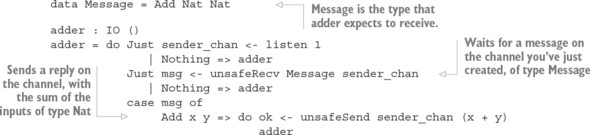
Similarly, the following listing shows the complete definition of main, which sends a message using unsafeSend and receives a reply of type Nat with unsafeRecv.
Listing 15.5. Complete definition of main (AdderChannel.idr)
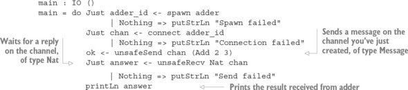
*AdderChannel> :exec main 5
This only works because you’ve ensured that main and adder agree on a communication pattern. When main sends a message on a channel, the adder process is expecting to receive a message on its corresponding channel, and vice versa.
15.1.3. Problems with channels: type errors and blocking
Channels provide a primitive method of setting up links between processes and sending messages across those links. The types of unsafeSend and unsafeRecv don’t, however, provide any kind of guarantees about how processes coordinate with each other. As a result, it’s easy to make a mistake.
For example, adder sends a Nat in reply to main, but what if main is expecting to receive a String?
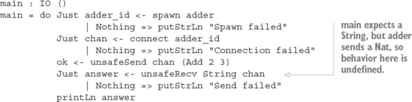
In this case, executing main will behave unpredictably, and will most likely crash, because at runtime there’s an inconsistency between the type of the message received and the expected type. Nothing in the types of unsafeSend and unsafeRecv explains how the sends and receives are coordinated between the two processes, so Idris is happy to accept main as valid even though the coordination is, in this case, incorrect.
A different problem occurs if the unsafeSend and unsafeReceive operations don’t correspond in each process. For example, main might send a second message on the same channel and expect a reply:
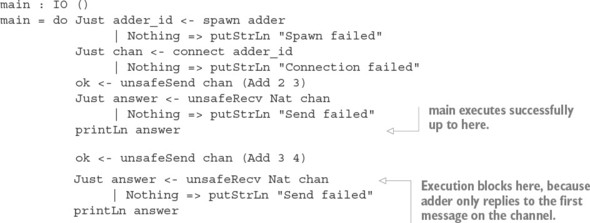
Although channels themselves are unsafe, you can use them as a primitive for defining type-safe communication. We’ll define a type for describing the coordination between communicating processes, and then write a run function that executes the description using the unsafe primitives. Even though, ultimately, you’ll need to use the primitives, you can encapsulate all the details in a single, descriptive type that you can then use for type-driven development of communicating systems.
15.2. Defining a type for safe message passing
In the Idris runtime system, concurrent processes run independently of each other. There’s no shared memory, and the only way processes can communicate with each other is by sending messages to each other. Because there’s no shared memory, there are no race conditions caused by accessing shared state simultaneously, but there are several other problems to consider:
- How can you ensure that the type of the message that main sends is the same type that adder expects to receive?
- What happens if main sends a message to adder, but adder doesn’t reply?
- What happens if adder has stopped running when main sends a message?
- How can you prevent the situation where main and adder are both waiting for a message from each other?
In this section, you’ll see how to solve these problems by defining a Process type, which allows you to describe well-typed communicating processes.
Support for types in concurrent programming has generally been quite limited in mainstream programming languages, with some exceptions, such as typed channels in Go. One difficulty is that, as well as the types of messages that a channel can carry, you also need to think about the protocol for message passing. In other words, as well as what to send (the type), you also need to think about when to send it (the protocol).
There has, nevertheless, been significant research into types for concurrent programming, most notably the study of session types that began with Kohei Honda’s 1993 paper “Types for Dyadic Interaction.” The type we’ll implement in this section is an instance of a session type with a minimal protocol where a client sends one message and then receives one reply. If you’re interested in exploring further, a recent (2016) paper, “Certifying Data in Multiparty Session Types” by Bernardo Toninho and Nobuko Yoshida, describes a more sophisticated way of using types in concurrent programs.
15.2.1. Describing message-passing processes in a type
Earlier, I described two problems with the primitive Channel type that make concurrent programming, in this primitive form, unsafe:
- There’s no way to check that a response to a request has the correct type.
- There’s no way to check the correspondence between sending and receiving messages in communicating processes.
We’ll solve both of these problems by defining a type for describing processes and then refining it as necessary to support the message-passing features we need.
To start, you can define a process type that supports IO actions, constructing pure values, and sequencing.
Listing 15.6. A type for describing processes (Process.idr)
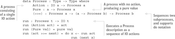
Using IO in Action
By using IO in Action, you can include arbitrary IO actions in processes, such as writing to the console or reading user input. This is a bit too general, because IO actions include, among other things, the unsafe communication primitives. You could restrict this by defining a more precise command type (see chapter 11 for an example), but we’ll stick with IO for this example.
At the moment, Process is nothing more than a wrapper for sequences of IO actions. The next step is to extend it to support spawning new processes. You can define a data type for representing processes that can receive a Message, using PID from System.Concurrency.Channels:
data MessagePID = MkMessage PID
Next, you can add a constructor to Process that describes an action that spawns a new process and returns the MessagePID of that process, if it was successful:
Spawn : Process () -> Process (Maybe MessagePID)You also need to extend run to be able to execute the new Spawn command. This spawns a new process using the spawn primitive and then returns a MessagePID containing the new PID:
run (Spawn proc) = do Just pid <- spawn (run proc) | Nothing => pure Nothing pure (Just (MkMessage pid))
Adding new constructors
Remember that after you’ve added the Spawn constructor, you can add the missing cases to run in Atom by pressing Ctrl-Alt-A with the cursor over the name run.
Next, you can add commands to allow processes to send messages to each other. In the previous examples, the main process sent requests of type Message and waited for corresponding replies of type Nat. You can encapsulate this behavior in a single Request command:
Request : MessagePID -> Message -> Process (Maybe Nat)
The reason for returning Maybe Nat, rather than Nat, is that you don’t have any guarantee that the process to which MessagePID refers is still running. When you run a Request, you’ll need to connect to the process that services the request, send it a message, and then wait for the reply:
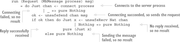
Encapsulating primitives in the Process type
You still need to use unsafeSend and unsafeRecv, but by encapsulating them in the Process data type, you know there’s only one place in your program where you use the unsafe primitives. You need to be careful to get this definition right, but once you do, you know that any message-passing program implemented in terms of the Process type will follow the message-passing protocol correctly.
The adder process waited for an incoming message, calculated a result, and sent a response back to the requester. You can encapsulate this behavior in a single Respond command:
Respond : ((msg : Message) -> Process Nat) -> Process (Maybe Message)
This takes a function as an argument, which, when given a message received from a requester, calculates the Nat to send back. It returns a value of type Maybe Message, which is either Nothing, if it didn’t process an incoming message, or of the form Just msg, if it processed an incoming message (msg). This is useful if you need to do any further processing with the incoming message, even after sending a response.
When you run the Respond command, you’ll wait for one second for a message and then, if there is a message, calculate the response and send it back:
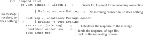
Alternative implementations for Respond
This implementation of the Respond case waits for 1 second if there’s no incoming message. An alternative, and more flexible, implementation might allow the user to specify a time-out. For example, if there’s no incoming request, it might not make sense to continue waiting if a process has other work to do.
Listing 15.7 shows how you can define adder and main using Process. We’ll call them procAdder and procMain to distinguish them from the earlier versions. In proc-Adder, you use Respond to explain how to respond to a Message, and in procMain you use Request to send a message to a spawned process.
Listing 15.7. Implementing a type-safe adder process (Process.idr)
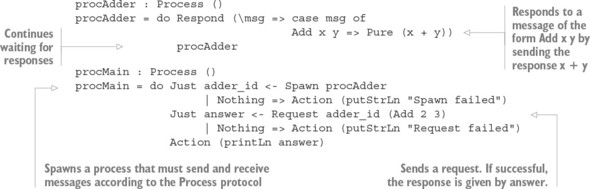
You can try this at the REPL, using run to translate procMain to a sequence of IO actions:
*Process> :exec run procMain 5
Unlike the previous version, procMain can’t expect to receive a String rather than a Nat, because the type of Request doesn’t allow it. You’ve also encapsulated the
communication protocol on a channel using Request and Respond, so you know that you won’t send or receive too many messages after creating a channel.As a first attempt, this is an improvement over the primitive implementation with Channel, but there are a number of ways you can improve it. For example, procAdder is not total:
*Process> :total procAdder Main.procAdder is possibly not total due to recursive path: Main.procAdder
This is potentially a problem, because a process that isn’t total may not successfully respond to requests. As a first refinement, you can modify the Process type, and correspondingly the definition of run, so that indefinitely running processes like proc-Adder are total.
15.2.2. Making processes total using Inf
As you saw in chapter 11, you can mark parts of data as potentially infinite using Inf:
Inf : Type -> Type
You can then say a function is total if it produces a finite prefix of constructors of a well-typed infinite result in finite time. In practice, this means that any time you use a value with an Inf type, it needs to be an argument to a data constructor or a nested sequence of data constructors.
You’ve seen various ways to use Inf to define potentially infinite processes in chapters 11 and 12. Here, you can use it to explicitly mark the parts of a process that loop by adding the following constructor to Process:
Loop : Inf (Process a) -> Process a
For reference, the next listing shows the current definition of Process, including Loop, defined in a new file, ProcessLoop.idr.
Listing 15.8. New Process type, extended with Loop (ProcessLoop.idr)
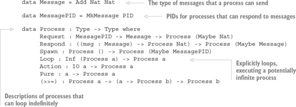
procAdder : Process () procAdder = do Respond (\msg => case msg of Add x y => Pure (x + y)) Loop procAdder
This version of procAdder is total:
*ProcessLoop> :total procAdder Main.procAdder is Total
By using an explicit Loop constructor, you can mark the infinite parts of a Process so that you can at least be sure that any infinite recursion is intended. Moreover, as you’ll see in the next section, it will allow you to refine Process further so that you can control exactly when a process is allowed to loop.
You’ll also need to extend run to support Loop. The simplest way is to execute the action directly:
run (Loop act) = run act
Unfortunately, this new definition of run isn’t total because the totality checker (correctly!) doesn’t believe that act is a smaller sequence than Loop act:
*ProcessLoop> :total run Main.run is possibly not total due to recursive path: Main.run, Main.run, Main.run
As with the infinite processes in chapter 11, you can define a Fuel data type to give an explicit execution limit to run. Every time you Loop, you reduce the amount of Fuel available. The following listing shows how you can extend run so that it terminates when it runs out of Fuel, following the pattern you’ve already seen in chapter 11.
Listing 15.9. New run function, with an execution limit (ProcessLoop.idr)
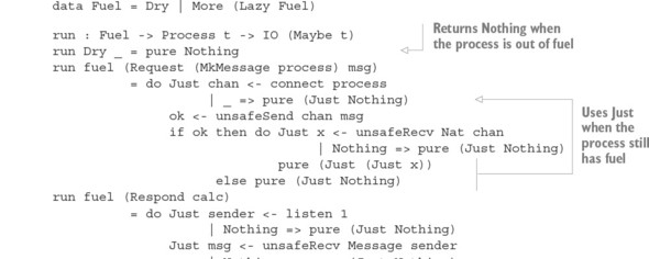
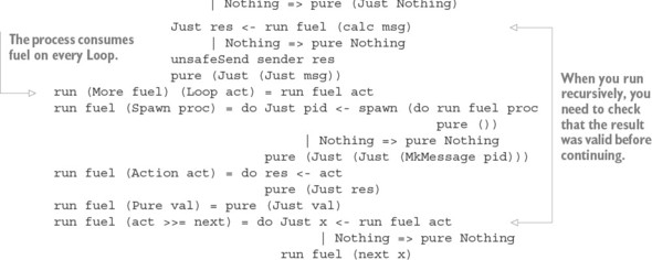
partial forever : Fuel forever = More forever
Using a single forever function to say how long an indefinite process is allowed to run means that you minimize the number of nontotal functions you need. Because run is total, you know that it will continue executing process actions as long as there are actions to execute. For convenience, you can also define a function for initiating a process and discarding its result:
partial runProc : Process () -> IO () runProc proc = do run forever proc pure ()
Then, you can try executing procMain as follows, which will display the answer 5 as before:
*ProcessLoop> :exec runProc procMain 5
Using Loop, you can write processes that loop forever and that are total by being explicit about when they loop. Unfortunately, though, there’s still no guarantee that a looping process will respond to any messages at all. For example, you could define procAdder as follows:
procAdderBad1 : Process () procAdderBad1 = do Action (putStrLn "I'm out of the office today") Loop procAdderBad1
Or even like this:
procAdderBad2 : Process () procAdderBad2 = Loop procAdderBad2Both of these programs type-check, and are both checked as total, but neither will respond to any messages because there’s no Respond command. In the case of proc-AdderBad2, it’s total because the recursive call to procAdderBad2 is an argument to the Loop constructor, so it will produce a finite prefix of constructors. Being total using Loop is, therefore, not enough to guarantee that a process will respond to a request.
The meaning of totality, in practice
Totality means that you’re guaranteed that a function behaves in exactly the way described by its type, so if the type isn’t precise enough, neither is the guarantee! With Process, the type isn’t precise enough to guarantee that a process contains a Respond command before any Loop.
Furthermore, the Process type is specific to the problem of writing a concurrent service to add numbers. What if you want to write different services? You don’t want to have to write a different Process type for every kind of service you might want to Spawn.
To solve these problems, you’ll need to refine the Process type in two more ways:
- In section 15.2.3, you’ll refine it to ensure that a server process responds to requests on every iteration of a Loop.
- In section 15.2.4, you’ll see how to use first-class types to allow Process to respond to any kind of message.
15.2.3. Guaranteeing responses using a state machine and Inf
In chapter 13, you saw how to guarantee that systems would execute necessary actions in the correct order by representing a state machine in a type. A server process like adder could be in one of several states, depending on whether or not it has received and processed a request:
- NoRequest—It has not yet serviced any requests.
- Sent—It has sent a response to a request.
- Complete—It has completed an iteration of a loop and is ready to service the next request.
Figure 15.3 illustrates how the Respond and Loop commands affect the state of a process.
Figure 15.3. A state transition diagram showing the states and operations in a server process. A process begins in the NoRequest state and must end in the Complete state, meaning that it has responded to at least one request.
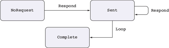
If you have a process that begins in the NoRequest state and ends in the Complete state, you can be certain that it has replied to a request, because the only way to reach the Complete state is by calling Respond. You can also be certain that it’s continuing to receive requests, because the only way to reach the Complete state is by calling Loop. By expressing the state of a process in its type, you can then make stronger guarantees about how that process behaves.
You can refine the type of Process to represent the states before and after the process is executed:
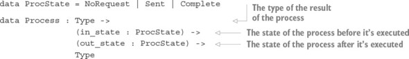
The states in the type give the preconditions and postconditions of a process. For example:
- Process () NoRequest Complete is the type of a process that responds to a request and then loops.
- Process () NoRequest Sent is the type of a process that responds to one or more requests and then terminates.
- Process () NoRequest NoRequest is the type of a process that responds to no requests and then terminates.
Listing 15.10 shows the refined Process, where the type of each command explains how it affects the overall process state. In this definition, where there’s no precondition on the state and no change in the state, the input and output states are both st.
Listing 15.10. Annotating the Process type with its input and output states (ProcessState.idr)
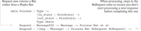
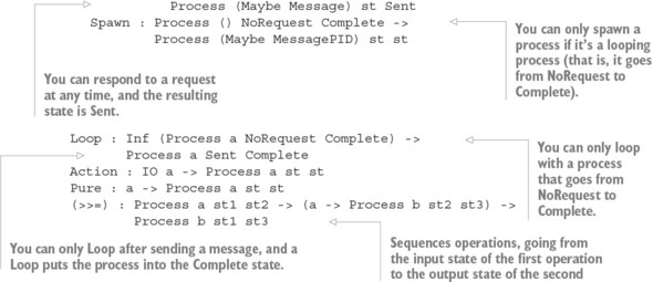
Return type of Request
Earlier, you sent requests of type Message and received responses of type Maybe Nat. You used Maybe because you had no guarantee that the service was still running, so the request could fail. Now you’ve set up the Process state so that services will always respond to requests. If you send a request, you’re guaranteed a response of type Nat in finite time.When you use this new definition, there’s no way for a function to invoke Loop unless the function can satisfy the precondition that it has sent a response to a request. Moreover, Loop is also the only way for a process to reach the Complete state. As a result, you can only invoke Loop on a process that’s guaranteed to be looping, because the process must begin in the NoRequest state and end in the Complete state.
You can still define procAdder as before, because each command satisfies the precondition, and its type now states that it must respond to a request and then loop:
procAdder : Process () NoRequest Complete procAdder = do Respond (\msg => case msg of Add x y => Pure (x + y)) Loop procAdder
The two incorrect versions defined earlier, however, no longer type-check, because the commands don’t satisfy the preconditions given by Process when you attempt to use them. For example, you can try the following definition:
procAdderBad1 : Process () NoRequest Complete procAdderBad1 = do Action (putStrLn "I'm out of the office today") Loop procAdder
Idris reports an error because there’s no Respond before the Loop:
ProcessState.idr:63:21: When checking right hand side of procAdderBad1 with expected type Process () NoRequest Complete When checking an application of constructor Main.>>=: Type mismatch between Process a Sent Complete (Type of Loop _) and Process () NoRequest Complete (Expected type) Specifically: Type mismatch between Sent and NoRequestThis error message means that when you call Loop, the process is supposed to be in the Sent state, but at this point it’s in the NoRequest state, not having sent any response yet. You’ll get a similar error message for the same reason with the following definition:
procAdderBad2 : Process () NoRequest Complete procAdderBad2 = Loop procAdderBad2
In order to execute programs using the refined Process, you’ll need to modify run and runProc. First, you need to modify their types:
run : Fuel -> Process t in_state out_state -> IO (Maybe t) runProc : Process () in_state out_state -> IO ()
The definitions mostly remain the same as the previous versions. The one change is in the definition of the Request case in run, now that you know a Request will always receive a reply in finite time:
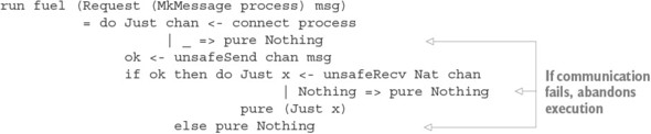
Return value of run
If run fails for any reason, it returns Nothing. Up to now, this could only happen if it ran out of Fuel. You’ve now set up Process so that senders and receivers are coordinated, so, at least in theory, communication can’t fail. If communication does fail, there’s either an error in the implementation of run or a more serious runtime error, so you can also return Nothing in this case.
You’ll also need to modify the type of procMain, to be consistent with the refined Process type. This type explicitly states that procMain isn’t intended to respond to any incoming requests because it ends in the NoRequest state:
procMain : Process () NoRequest NoRequest
It’s convenient to define type synonyms for clients, like procMain, and for services, like procAdder. They both use Process, but they differ in how they affect the state of the process:
Service : Type -> Type Service a = Process a NoRequest Complete Client : Type -> Type Client a = Process a NoRequest NoRequestThe following listing shows the refined definitions of procAdder and procMain using these type synonyms for client and server processes.
Listing 15.11. Refined definitions of procAdder and procMain (ProcessState.idr)
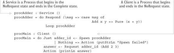
If you try this at the REPL, you’ll see that it displays 5 as before:
*ProcessState> :exec runProc procMain 5
You now have a definition of Process with the following guarantees, ensured by the preconditions and postconditions in the definition of Process:
- All requests of type Message are sent responses of type Nat.
- Every process started with Spawn is guaranteed to loop indefinitely and respond to requests on every iteration.
- Therefore, every time a process sends a Request to a service started with Spawn, it will receive a response in finite time as long as the service is defined by a total function.
This means you can write type-safe concurrent programs that can’t deadlock, because every request is guaranteed to receive a response eventually. But at this stage, it only allows you to write one kind of service—one that receives a Message and sends back a Nat. It would be far more useful if you could define generic message-passing processes with user-defined interactions between the sender and receiver. As you’ll see, you can achieve this with a final small refinement to Process.
15.2.4. Generic message-passing processes
When a process receives a request of the form Add x y, it sends back a response of type Nat. You can express this relationship between the request and the response types in a type-level function:
AdderType : Message -> Type AdderType (Add x y) = Nat
This function describes the interface that Process supports: if it receives a message of the form Add x y, it will send a response of type Nat. You could define other interfaces this way; for example, the following listing gives a description of an interface to a process that responds to requests to perform operations on lists.
Listing 15.12. Describing an interface for List operations
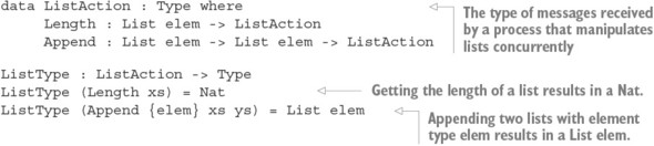
In general, an interface to a process is a function like AdderType or ListType that calculates a response type from a request. Instead of defining a specific type that processes can send and receive, you can include the interface as part of a process’s type by adding an additional argument for the interface, as figure 15.4 shows.
Figure 15.4. A refined Process type, including the interface that the process responds to as part of the type
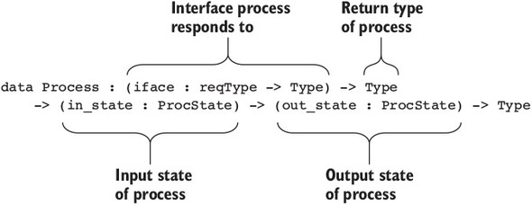
Request type of Process
The iface argument to Process includes a type variable, reqType. This is an implicit argument, and it defines the type of messages the process can receive. Idris will infer reqType from the iface argument. For example, in procAdder, iface is AdderType, so reqType must be Message.
We’ll come to the refined definition of Process shortly. Once it’s defined, the procAdder service will respond to an interface defined by AdderType:
procAdder : Process AdderType () NoRequest Complete
Some processes, like procMain, don’t respond to any requests. You can make this explicit in the type by defining their interfaces as follows:
NoRecv : Void -> Type NoRecv = const VoidRemember from chapter 8 that Void is the empty type, with no values. Because you can never construct a value of type Void, a process that provides a NoRecv interface can never receive a request. You can use it in the following type for procMain:
procMain : Process NoRecv () NoRequest NoRequest
You’ll also need to redefine the type synonyms Service and Client to include the interface description. A Service has an interface, but a Client receives no requests:
Service : (iface : reqType -> Type) -> Type -> Type Service iface a = Process iface a NoRequest Complete Client : Type -> Type Client a = Process NoRecv a NoRequest NoRequest
When you create a new process, you get a PID for the new process as a MessagePID. You should only send messages to a process when the messages match the interface of that process, so you can refine MessagePID to include the interface it supports in its type:
data MessagePID : (iface : reqType -> Type) -> Type where MkMessage : PID -> MessagePID iface
Now, if you have a PID of type MessagePID AdderType, you know that you can send it messages of type Message, because that’s the input type of AdderType.
Putting all of this together, you can refine Process to describe its own interface and to be explicit about when it’s safe to send a request of a particular type to another Process. The next listing shows the refined types for Request, Respond, and Spawn.
Listing 15.13. Refining Process to include its interface in the type, part 1 (ProcessIFace.idr)
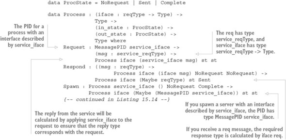
The following listing completes the refined definition of Process, adding Loop, Action, Pure, and (>>=). In each case, all you need to do is add an iface argument to Process.
Listing 15.14. Refining Process to include its interface in the type, part 2 (ProcessIFace.idr)
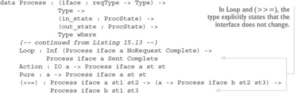
Finally, you need to update run and runProc for the refined Process definition. Listing 15.15 shows the changes you need to make to run. You need only modify the cases for Request and Respond to be explicit about the types of messages a process expects to receive.
Listing 15.15. Updating run for the refined Process (ProcessIFace.idr)
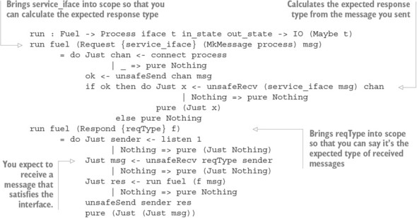
For runProc, you need only change its type to add the iface argument to Process:
partial runProc : Process iface () in_state out_state -> IO () runProc proc = do run forever proc pure ()When designing data types, especially types that express strong guarantees like Process, it’s often a good idea to begin by trying to solve a specific problem before moving on to a more general solution. Here, we started with a type for Process that only supported specific message and response types (Message and Nat). Only after that worked did we use type-level functions to make a generic Process type.
15.2.5. Defining a module for Process
Once you’ve defined a generic type, it’s useful to define a new module to make that type and its supporting functions available to other users. We’ll define a new module, ProcessLib.idr, that defines Process and supporting definitions and exports them as necessary.
The next listing shows the overall structure of the module, omitting the definitions but adding export modifiers to each declaration.
Listing 15.16. Defining Process in a module, omitting definitions (ProcessLib.idr)
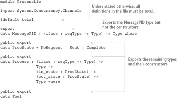
The complete definitions are the same as those you’ve already seen for MessagePID, ProcState, Process, and Fuel. Remember from chapter 10 that for data declarations, an export modifier can be one of the following:
- export—The type constructor is exported but not the data constructors.
- public export—The type and data constructors are exported.
The following listing shows how you can export the supporting functions.
Listing 15.17. Supporting function types for Process, omitting definitions (ProcessLib.idr)
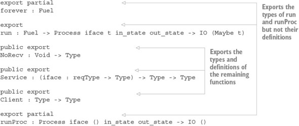
- export—The type is exported but not the definition.
- public export—The type and definition are exported.
Unless there’s a specific reason to export a definition as well as a type, it’s better to use export, hiding the details of the definition. Here, you use public export for Client and Service because these are type synonyms, and other modules will need to know that these are defined in terms of Process.
Now that you’ve defined Process and a separate ProcessLib module that exports the relevant definitions, we can try more examples. To conclude this section, we’ll look at two examples of implementing concurrent programs using this generic Process type. First, we’ll implement a process using ListType, which was defined earlier in listing 15.12, and then we’ll look at a larger example using concurrency to run a process in the background to count words in a file.
15.2.6. Example 1: List processing
To demonstrate how you can use Process to define services other than procAdder, we’ll start with a service that responds to requests to carry out functions on List. The interface of the service is defined by a ListType function. It provides two operations: Length and Append.
data ListAction : Type where Length : List elem -> ListAction Append : List elem -> List elem -> ListAction ListType : ListAction -> Type ListType (Length xs) = Nat ListType (Append {elem} xs ys) = List elem We’ll define a procList service that responds to requests on this interface. It has the following type: procList : Service ListType ()
You can define procList incrementally, taking the following steps:
- Define, type—As with procAdder, you can implement procList as a loop that responds to a request on each iteration:
procList : Service ListType () procList = do Respond (\msg => ?procList_rhs) Loop procList
Looking at the ?procList_rhs type here, you can see that the type you need to produce is calculated from the msg you receive:msg : ListAction -------------------------------------- procList_rhs : Process ListType (ListType msg) NoRequest NoRequest
- Define— Because the type you need to produce depends on the value of msg, you can continue the definition with a case statement, inspecting msg:
procList : Service ListType () procList = do Respond (\msg => case msg of case_val => ?procList_rhs) Loop procList
Case splitting on case_val produces this:procList : Service ListType () procList = do Respond (\msg => case msg of Length xs => ?procList_rhs_1 Append xs ys => ?procList_rhs_2) Loop procList
- Type, refine—For ?procList_rhs_1, if you check the type, you’ll see that you need to produce a Nat for the result of Length xs:
msg : ListAction a : Type xs : List elem -------------------------------------- procList_rhs_1 : Process ListType Nat NoRequest NoRequest
You can refine ?procList_rhs_1 as follows:procList : Service ListType () procList = do Respond (\msg => case msg of Length xs => Pure (length xs) Append xs ys => ?procList_rhs_2) Loop procList
- Refine— To refine ?procList_rhs_2, you need to provide a List elem, and you can complete the definition as follows:
procList : Service ListType () procList = do Respond (\msg => case msg of Length xs => Pure (length xs) Append xs ys => Pure (xs ++ ys)) Loop procList
Listing 15.18. A main program that uses the procList service (ListProc.idr)
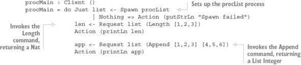
You can try this at the REPL as follows:
*ListProc> :exec runProc procMain 3 [1, 2, 3, 4, 5, 6]
Like procAdder, procList loops, waiting for incoming requests, and processes them as necessary, but it doesn’t do any other computation while waiting for a request. Concurrent processes become far more useful if, rather than spending their time idling and waiting for requests from other processes, they also do some computation. In the next example, you’ll see how to do this.
15.2.7. Example 2: A word-counting process
When you define services, you can define separate requests for initiating an action and getting the result of that action. For example, if you’re defining a word-count service, you could allow a client to take the following steps:
- Send a request to a word-count service to load a file and count the number of words in the file.
- While the word-count service is processing, the client continues its own work, such as reading input and producing output.
- Send a second request to the word-count service to ask how many words were in the file.
In this example, you’ll define the word-count service around the WCData record and doCount function defined in listing 15.19. This function takes the contents of a file, in a String, and produces a structure containing the numbers of words and lines in that content.
Listing 15.19. A small function to count the number of words and lines in a String (WordCount.idr)
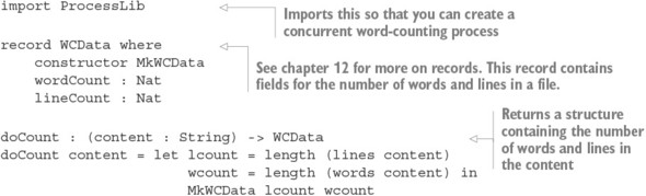
*WordCount> doCount "test test\ntest" MkWCData 2 3 : WCData
The goal is to implement a process that provides word counting as a service. Rather than loading and counting the words in a single request, you can provide two commands:
- CountFile—Given a filename, loads that file and counts the number of words in it
- GetData—Given a filename, returns the WCData structure for that file, as long as the file has already been processed with CountFile
Rather than returning the WCData structure itself, CountFile will return immediately and continue loading the file in a separate process. That is, one request begins the task and another retrieves the result. This will allow the requester to continue its own work while the word-count service is processing the file. The following listing shows the interface and a skeleton definition for the word-count service.
Listing 15.20. Interface for the word-count service (WordCount.idr)
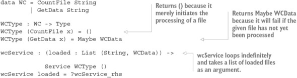
We’ll come to the definition of wcService in a moment. The next listing shows how you can invoke it and continue to execute interactive actions in the foreground while wcService is processing a file in the background.
Listing 15.21. Using the word-count service (WordCount.idr)
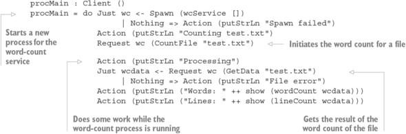
Listing 15.22 presents an incomplete implementation of wcService that shows how it responds to the commands CountFile and GetData. Two parts of the definition are missing:
- Loading and processing the requested file
- Looping, with the new file information added to the input, loaded
Listing 15.22. Responding to commands in wcService (WordCount.idr)
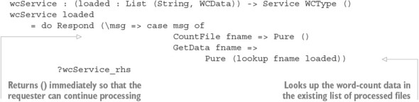
To process the input, you can look at the return value from Respond. Remember that Respond has the following type:
Respond : ((msg : reqType) -> Process iface (iface msg) NoRequest NoRequest) -> Process iface (Maybe reqType) st Sent
The return value from Respond, of type Maybe reqType, tells you which message, if any, was received. If wcService received a CountFile command, it could load and process the necessary file before processing its next input.
The next listing shows a further refinement of wcService, still including a hole for the function that processes the file.
Listing 15.23. Incomplete implementation of wcService (WordCount.idr)
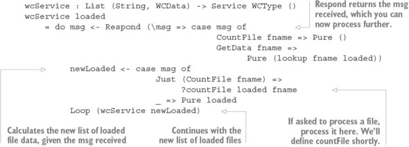
To see what you need to do to complete wcService, you can check the type of ?countFile:
loaded : List (String, WCData) fname : String msg2 : Maybe WC st2 : ProcState a : Type -------------------------------------- countFile : List (String, WCData) -> String -> Process WCType (List (String, WCData)) Sent Sent
countFile needs to be a function that takes the current list of processed file data and a filename, and then returns an updated list of processed file data. The next listing shows how to define it using doCount, defined earlier, to process the file’s contents.
Listing 15.24. Loading a file and counting words (WordCount.idr)
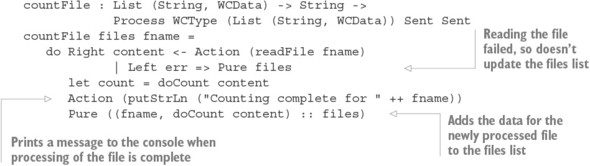
Updating the hole for countFile
Remember that you need to define countFile before you use it in wcService. Once you’ve defined countFile, don’t forget to replace the ?countFile hole with a call to countFile.
Now that you’ve defined countFile, you can try executing procMain, which starts wcService, asks to count the words in a file, test.txt, and then displays the result. You’ll need to create a test.txt file with content like the following:
test test test test test test test
You can execute procMain at the REPL as follows:
With Process, you’ve defined a type that allows you to describe concurrently executing processes and to explain how processes can send each other messages safely, following a protocol:
- A service must respond to every message it receives, on a specific interface, and continue responding in a loop.
- A client can then send a message to a process, with the correct interface, and be sure of receiving a reply of the correct type.
This doesn’t solve all possible concurrent programming problems, but you’ve defined a type that encapsulates the behavior of one kind of concurrent program. If a function describing a Process type-checks and is total, you can be confident that it won’t deadlock and that all requests will receive replies. If you later refine Process further, such as by allowing more-sophisticated descriptions of interactions between processes, you’ll be able to implement more-sophisticated models of concurrent programs.
15.3. Summary
- Concurrent programming involves multiple processes executing simultaneously.
- Processes in Idris cooperate with each other by sending messages.
- The System.Concurrency.Channels library provides primitive, but unsafe, operations for message passing.
- Primitive operations are unsafe because they provide no guarantees about when processes send and receive messages, or about the correspondence between the types of sent and received messages.
- You can define a type for describing safe message-passing processes, implemented using Channel as a primitive.
- Using Inf, you can guarantee that looping processes continue to perform IO actions.
- By defining a state machine in the type, you can be sure that a process will respond to messages on every iteration of a loop.
- The type of a process can be generic and describe the types of messages to which a process will respond.
Appendix A. Installing Idris and editor modes
This appendix explains how to install Idris. There are prebuilt binary distributions for Mac and Windows, or you can install from source on any Unix-like operating system. It also describes how to install the Idris mode in the Atom text editor.The Idris compiler and environment
At the time of writing, Idris is available as a binary distribution for Windows and Mac OS from http://idris-lang.org/download. This includes the compiler and REPL, along with the Prelude, base libraries, and a variety of contributed libraries that support various data structures, networking, and programming with side effects.
In the following sections, I’ll describe how to install Idris either as binaries or from source. In either case, to check that Idris has installed successfully, you can run idris --version, which reports which Idris version is installed:
$ idris --version 1.0
Mac OS
The latest version of Idris is always available as a binary package, downloadable at http://idris-lang.org/pkgs/idris-current.pkg. To be able to compile it and run your programs, you’ll also need to install Xcode, which is available from the App Store.
To install Idris, therefore, you can follow these steps:- Download idris-current.pkg.
- Ensure that Xcode is installed from the App Store.
- Open idris-current.pkg and follow the instructions. This will install the Idris binary to /usr/local/bin/idris.
You can also install the latest version via Homebrew (http://brew.sh/):
$ brew install idris
Windows
Prebuilt binaries of Idris are available from https://github.com/idris-lang/Idris-dev/wiki/Windows-Binaries. These binaries include everything necessary for compiling and running Idris programs.
Unix-like platforms, installing from source
Idris is implemented in Haskell, and a source distribution is available from the Haskell package manager, Hackage (http://hackage.haskell.org/). This is a good option if you’re using an operating system for which there are no binary releases available, or if you need more control over how Idris is set up.
To install it, follow these steps:
- Install the Haskell Platform, available from www.haskell.org/downloads.
- The Haskell Platform includes a command-line tool, cabal, for installing applications and libraries from the central Hackage repository. Assuming you’re in a Unix-like environment, you can install Idris to an executable at /usr/local/bin/idris with the following commands:
$ cabal update $ cabal install idris --program-prefix=/usr/local
Editor modes
In this section, I’ll describe how to install the Idris mode for type-driven interactive editing in the Atom text editor, used throughout this book. I’ll also give you some pointers to editor modes for Emacs and Vim.
Atom
Atom is available for all major platforms from http://atom.io/. You can install the extension for editing Idris programs as follows:
- Go to Preferences.
- Go to the Install tab.
- Search for the language-idris package.
- There should be one search result. Click the Install button for this result.
- You’ll need to tell the language-idris package where the Idris binary is installed. To do this, first go to the Packages tab.
- Click on Settings in the language-idris box.
- Under the Settings heading, enter the path where the Idris binary is installed. On this page, you can also change the keyboard shortcuts and various other features.
Other editors
At the time of writing, editor modes are also available for Vim and Emacs:
- Vim extension—https://github.com/idris-hackers/idris-vim
- Emacs mode—https://github.com/idris-hackers/idris-mode
In each case, installation, configuration, and usage instructions are provided.
Appendix B. Interactive editing commands
Throughout the book, I describe the interactive construction of Idris programs via editing commands in Atom. The following table summarizes these commands for easy reference.
Table 1. Interactive editing commands in Atom
| Shortcut | Command | Description |
|---|---|---|
| Ctrl-Alt-A | Add definition | Adds a skeleton definition for the name under the cursor |
| Ctrl-Alt-C | Case split | Splits a definition into pattern-matching clauses for the name under the cursor |
| Ctrl-Alt-D | Documentation | Displays documentation for the name under the cursor |
| Ctrl-Alt-L | Lift hole | Lifts a hole to the top level as a new function declaration |
| Ctrl-Alt-M | Match | Replaces a hole with a case expression that matches on an intermediate result |
| Ctrl-Alt-R | Reload | Reloads and type-checks the current buffer |
| Ctrl-Alt-S | Search | Searches for an expression that satisfies the type of the hole name under the cursor |
| Ctrl-Alt-T | Type-check name | Displays the type of the name under the cursor |
| Ctrl-Alt-W | with block insertion | Adds a with block after the current line, containing a new pattern-matching clause with an extra argument |
Appendix C. REPL commands
The Idris read-eval-print loop (REPL) provides several commands for evaluating and inspecting expressions and types, compiling programs, and searching documentation, among other things. I introduce several of these throughout the book; the following table lists the most commonly used commands, but there are several others available. For more details, type :? at the REPL.Table 1. Idris REPL commands
| Command | Arguments | Description |
|---|---|---|
| <expression> | None | Displays the result of evaluating the expression. The variable it contains the result of the most recent evaluation. |
| :t | <expression> | Displays the type of the expression. |
| :total | <name> | Displays whether the function with the given name is total. |
| :doc | <name> | Displays documentation for name. |
| :let | <definition> | Adds a new definition. |
| :exec | <expression> | Compiles and executes the expression. If none is given, compiles and executes main. |
| :c | <output file> | Compiles to an executable with the entry point main. |
| :r | None | Reloads the current module. |
| :l | <filename> | Loads a new file. |
| :module | <module name> | Imports an extra module for use at the REPL. |
| :printdef | <name> | Displays the definition of name. |
| :apropos | <word> | Searches function names, types, and documentation for the given word. |
| :search | <type> | Searches for functions with the given type. |
| :browse | <namespace> | Displays the names and types defined in the given namespace. |
| :q | None | Exits the REPL. |
Appendix D. Further reading
This appendix lists several other resources through which you can learn more about functional programming, types, and Idris’ theoretical foundations. The resources are grouped by topic, with a brief comment on each.
Functional programming in Haskell
Idris is heavily inspired by Haskell, including its syntax, language features, and many of its standard libraries. In particular, Idris interfaces are closely related to Haskell type classes. If you’d like to learn about Haskell in more depth, you can take a look at the following books:
- Learn Haskell by Will Kurt (Manning, 2017) covers Haskell and functional programming concepts, including several practical examples, with particular emphasis on Haskell’s type system.
- Programming in Haskell, 2nd ed. by Graham Hutton (Cambridge University Press, 2016) introduces the core features of Haskell and pure functional programming, and it covers many of the more advanced features of Haskell.
- Thinking Functionally with Haskell by Richard Bird (Cambridge University Press, 2014) teaches programming from first principles using Haskell, particularly emphasizing techniques for reasoning mathematically about programs.
Other languages and tools with expressive type systems
Several other languages have arisen as a result of academic research into using types to reason about program correctness. These are some examples:
- Agda (http://wiki.portal.chalmers.se/agda/pmwiki.php)—Supports type-driven development using dependent types in the same way as Idris, but with a stronger emphasis on theorem proving.
- F* (www.fstar-lang.org/)—A functional programming language that aims to support program verification using refinement types, which are types augmented with a predicate that describes properties of values in that type.
- Coq (https://coq.inria.fr/)—A proof management system based on dependent types with support for extracting functional programs from proofs.
Theoretical foundations
Idris is based on decades of research in dependent type theory. You can learn more about the theoretical foundations from the following sources:
- Type Theory and Functional Programming by Simon Thompson (Addison Wesley, 1991). This book is now out of print, but it’s available online from the author’s website (www.cs.kent.ac.uk/people/staff/sjt/TTFP/). It provides an accessible introduction to type theory, including its foundations and applications.
- Software Foundations by Benjamin Pierce et al. (2016; www.cis.upenn.edu/~bcpierce/sf/current/index.html). This is a course on the mathematical underpinnings of software, from first principles, using Coq. It’s instructive to reproduce the examples in Idris!
- Types and Programming Languages by Benjamin Pierce (MIT Press, 2002). This textbook provides a comprehensive introduction to type systems and the basic theory of programming languages.
- “Propositions as Types” by Philip Wadler (Communications of the ACM, December 2015; http://cacm.acm.org/magazines/2015/12/194626-propositions-as-types). This paper gives a deep but accessible account of the relationship between logic and programming languages, and in particular the idea that a type in a programming language corresponds to a logical proposition and that a program corresponds to a proof of that proposition.
Total functional programming
Throughout this book, I talk about the value of writing total functions, and in chapter 10 I introduce views, which provide one way of writing total functions. There are several other techniques, some of which are described in the following papers:
- “Elementary Strong Functional Programming” by David Turner (Lecture Notes in Computer Science 1022 (1995):1–13). In this paper, David Turner argues in favor of writing total functions, describing many of the benefits and giving some basic techniques for writing total functions.
- “Why Dependent Types Matter” by Thorsten Altenkirch, Conor McBride and James McKinna (2004). This paper, available online (www.cs.nott.ac.uk/~psztxa/publ/ydtm.pdf), describes an earlier dependently typed language, Epigram, emphasizing the importance of totality in dependently typed programming.
- “Modelling general recursion in type theory” by Ana Bove and Venanzio Capretta (Mathematical Structures in Computer Science 15 (2005):671–708). Here, the authors describe a way to formalize recursive programs by defining a data type to describe the computational structure of the program.
Types for concurrency
Chapter 15 presents a way of implementing type-safe concurrent programs, but it uses a very simplified form of concurrent program. You can learn more about types for concurrent programming by reading about session types, first described by Kohei Honda in 1993. There are many sources, but the following papers provide a starting point:
- “Types for Dyadic Interaction” by Kohei Honda (Lecture Notes in Computer Science 715 (1993):509–523). This paper introduced the concept of session types, describing a type system for encoding interactions between two processes.
- “Multiparty Asynchronous Session Types” by Kohei Honda, Nobuko Yoshida, and Marco Carbone (Principles of Programming Languages, 2008). This paper extends the idea of session types to communicating systems with more than two participants.
Appendix
The Idris read-eval-print loop (REPL) provides several commands. The most common commands, listed below, are introduced over the course of this book.
| Command | Arguments | Description |
|---|---|---|
| <expression> | None | Displays the result of evaluating the expression. The variable it contains the result of the most recent evaluation. |
| :t | <expression> | Displays the type of the expression. |
| :total | <name> | Displays whether the function with the given name is total. |
| :doc | <name> | Displays documentation for name. |
| :let | <definition> | Adds a new definition. |
| :exec | <expression> | Compiles and executes the expression. If none is given, compiles and executes main. |
| :c | <output file> | Compiles to an executable with the entry point main. |
| :r | None | Reloads the current module. |
| :l | <filename> | Loads a new file. |
| :module | <module name> | Imports an extra module for use at the REPL. |
| :printdef | <name> | Displays the definition of name. |
| :apropos | <word> | Searches function names, types, and documentation for the given word. |
| :search | <type> | Searches for functions with the given type. |
| :browse | <namespace> | Displays the names and types defined in the given namespace. |
| :q | None | Exits the REPL. |
Appendix
Atom commands used for the interactive construction of Idris projects featured in this book are detailed below.
| Shortcut | Command | Description |
|---|---|---|
| Ctrl-Alt-A | Add definition | Adds a skeleton definition for the name under the cursor |
| Ctrl-Alt-C | Case split | Splits a definition into pattern-matching clauses for the name under the cursor |
| Ctrl-Alt-D | Documentation | Displays documentation for the name under the cursor |
| Ctrl-Alt-L | Lift hole | Lifts a hole to the top level as a new function declaration |
| Ctrl-Alt-M | Match | Replaces a hole with a case expression that matches on an intermediate result |
| Ctrl-Alt-R | Reload | Reloads and type-checks the current buffer |
| Ctrl-Alt-S | Search | Searches for an expression that satisfies the type of the hole name under the cursor |
| Ctrl-Alt-T | Type-check name | Displays the type of the name under the cursor |
| Ctrl-Alt-W | with block insertion | Adds a with block after the current line, containing a new pattern-matching clause with an extra argument |
Index
[SYMBOL][A][B][C][D][E][F][G][H][I][J][L][M][N][O][P][Q][R][S][T][U][V][W][Z]
SYMBOL
_ (underscore), 2nd, 3rd
:: operator, 2nd, 3rd
:printdef command
:r command
. function
/= method, 2nd
%default total annotation
+ operator
++ operator, 2nd
= type
== operator, 2nd, 3rd
>>= operator
$ operator, 2nd
$= operator
A
absurd function
accumulating parameter
Add command
addCorrect
addDownvote function
adder function, 2nd
AdderType function
addition function
addPositives
addToData function
addToStore function, 2nd, 3rd
addUpvote function
addWrong function
allLengths function, refining type of
anonymous functions
Append operation
AppendVec.idr file
Applicative interface
defining for State
generic do notation using
arguments
auto-implicit
defining functions with variable numbers of
addition function
printf function
arithInputs, 2nd
arithmetic notation
arithmetic quiz example
infinite lists
infinite processes
state
executing quiz
implementing quiz
nested records
updating record field values
updating record fields by applying functions
ATM example
defining states
defining type for
refining preconditions using auto-implicits
simulating at console
ATMCmd type
Atom, 2nd
commands
data types and patterns
defining functions by pattern matching
auto keyword
auto-implicits
overview
refining preconditions using
B
Bind constructor
Bool type
Booleans
bound implicit arguments
bracketing
built-in types, 2nd
C
cabal tool, Haskell
canonical constructors
case block
case expressions, using in types
case splitting, 2nd, 3rd
case statement
cast function, 2nd
Cast interface, converting between types with
catchall case
Channels library
character literals
checkEqNat function, 2nd, 3rd, 4th
Closed state
Command type
comments
communication pattern
composite types
lists
functions with
overview
tuples
concurrent programming
connect
Connected state
ConsoleIO programs
constants
constrained generic types
comparisons with Eq and Ord
constrained implemen-tations
default method definitions
defining Eq constraint
Ord
testing for equality with Eq
interfaces defined in Prelude
Cast
defining numeric types
Show
interfaces parameterized by Type -> Type
Foldable
Functor
Monad and Applicative
constrained types
control flow
pattern-matching bindings
producing pure values in interactive definitions
writing interactive definitions with loops
Control.Monad.State, 2nd
correct function
CountFile command
countFrom function, 2nd
covering function, 2nd
cycle function
D
data abstraction
data store
Traversing store's contents with views
Data.List.Views module
Data.Primitives.Views, 2nd
DataStore type
refining
using records for
deadlock
Dec type
decEq function
decidability
Dec
DecEq
decreasing argument
Delay function, 2nd
dependent state machines
describing rules in types
defining abstract game state and operations
defining concrete game state
defining type for game state
implementing game
running game
errors in state transitions
security properties in types
defining states
defining type
refining preconditions using auto-implicits
simulating at console
dependent types
defining
defining vectors
indexing vectors with bounded numbers
vehicle classification example
reading and validating
dependent pairs
reading vectors from console
reading vectors of unknown length
validating vector lengths
describeHelper function, 2nd
describeListEnd, 2nd
DivBy
Do constructor
do keyword
do notation, 2nd, 3rd
extending for infinite processes
sequencing commands with
sequencing expressions with Maybe type
using Monad and Applicative
doAdd
doCount function
door operations example
interactive development of sequences of operations
modeling door as a type
representing failure
verified, error-checking, door-protocol description
DoorClosed state, 2nd, 3rd
DoorCmd type, 2nd, 3rd
DoorOpen state, 2nd, 3rd
doorProg, 2nd
DoorResult type
DoorState
E
Effects library
Elem predicate
auto-implicit arguments
deciding membership of vectors
guaranteeing a value is in vectors
removing elements from Vect, 2nd
Emacs mode
empty function
empty type, 2nd
enumerated types, defining
Eq constraint
Eq interface
constrained implementations
default method definitions
defining using interfaces and implementations
testing for equality
Eq ty constant
EqNat type, 2nd
equal expressions
equality types
decidability
Dec
DecEq
empty type
guaranteeing equivalence of data with
= type
exactLength, 2nd
expressing equality of Nats as a type
manipulating equalities
testing for equality of Nats
reasoning about equality
appending vectors
delegating proofs and rewriting to holes
reversing vectors
rewrite construct
type checking and evaluation
equalSuffix function
evalState
exactLength function, 2nd, 3rd
ExactLength.idr file
execState
export modifier
Expr type
F
Face type
False value
filterKeys
Fin argument, indexing with bounded numbers
Finished type
finite prefix
first-class types
defining functions with variable numbers of arguments
addition function
printf function
schemas
DataStore type
displaying entries in store
holes
parsing entries according to
sequencing expressions with Maybe using do notation
updating
type-level functions
type synonyms
using case expressions in types
with pattern matching
Foldable interface, reducing structure using
Force function, 2nd
forever function, 2nd, 3rd
format string
Format type
Fractional interface
fromInteger method
Fuel type, 2nd
function definitions
local
overview
functions, 2nd
anonymous
defining by pattern matching
defining with variable numbers of arguments
addition function
Formatted output, a type-safe printf function
higher-order
local definitions
partial
partially applying
total, 2nd, 3rd
type-level
type synonyms
using case expressions in types
with pattern matching
types of
constrained
overview
variables in
using implicit arguments in
writing generic
Functor interface, 2nd
applying functions across structure with
defining for State
G
GameLoop type, 2nd, 3rd
GameState
generic types, defining
get command
GetData command
getEntry command
GetLine command, 2nd
getPrefix function, 2nd
GetRandom
GetStr command
getStringOrInt
getValues function
global state
greet function
guess function
guessing game example
defining abstract game state and operations
defining concrete game state
defining type for game state
implementing
running
H
Hangman guessing game example
completing top-level game implementation
deciding input validity
predicate for validating user input
processing guesses
representing game's state
top-level game function
Haskell
headUnequal
helper function
Here value
hierarchical namespaces
higher-order functions
holes
correcting compilation errors using
delegating proofs and rewriting to
Homebrew
I
Idris programming language
as pure functional programming language
partial and total functions
purity and referential transparency
side-effecting programs
checking types
comments
compiling and running programs
composite types
functions with lists
lists
tuples
editor modes
Atom
other editors
first-class types
functions
anonymous
higher-order
local definitions
partially applying
types and definitions of
writing generic with constrained types
writing generic with variables in types
holes
installing compiler and environment
Mac OS
Unix-like platforms
Windows
interactivity
REPL (read-eval-print loop)
types
Booleans
characters and strings
converting
numeric
whitespace
implicit arguments
bound and unbound
need for
using in functions
impossible keyword
Inf ty type
Inf type, 2nd
guaranteeing responses using state machine and
making processes total using
infinite lists
arithmetic quiz example
labeling elements in
processing
producing
Stream data type
total functions
infinite processes
arithmetic quiz example
describing
executing
extending do notation for
generating infinite structures using Lazy types
InfIO type
infix operator, 2nd
InfList
input and output processing
control flow
pattern-matching bindings
producing pure values in interactive definitions
writing interactive definitions with loops
IO generic type
>>= operator
do notation
evaluating and executing interactive programs
reading and validating dependent types
dependent pairs
reading vectors from console
reading vectors of unknown length
validating vector lengths
input function
Integral interface
interactive data store
interactively maintaining state in main
parsing user input
processing commands
representing store
interactive operations
interactive programming
control flow
reading and validating dependent types
with IO generic type
interface declarations
interfaces
defined in Prelude
Cast
defining numeric types
Show
generic comparisons
constrained implementations
default method definitions
defining Eq using interfaces and implementations
Ord
testing for equality with Eq
parameterized by Type -> Type
Foldable
Functor
Monad and Applicative
IO actions, 2nd, 3rd
IO Finished
IO generic type
>>= operator
do notation
evaluating and executing interactive programs
isInt
isList function
isSuffix function
isValidString, 2nd
it variable
items function
iterate function
J
L
labelFrom function
labelWith function, 2nd
language-idris package
Lazy annotation
Lazy types, generating infinite structures using
Length operation
let construct
linear congruential generator
List Char
List elem
listen
ListLast, 2nd
lists
functions with
matching last item in
reversing
snoc
ListType function
local mutable state
local state
logOpen function
Loop constructor
loopPrint function, 2nd
loops, writing interactive definitions with
M
MachineCmd, 2nd
main function
interactively maintaining state in main
overview, 2nd
map function
matrices
arithmetic involving
functions
operations and types
transposing
Matter type
Maybe elem
Maybe type, using do notation
maybeAdd function
membership tests
auto-implicit arguments
deciding membership of vectors
guaranteeing a value is in vectors
removing elements from Vect, 2nd
merge sorting
mergeSort function, 2nd, 3rd
MessagePID
method declarations
MkData
MkWordState argument
modules, in Idris
Monad interface
defining for State
generic do notation using
MonadState interface
mutable state
representing using pairs
State type
tree-traversal example
tree-traversal with State
mutual block
myReverse function, 2nd
myReverseHelper function
N
namespaces
Nats
expressing equality of as a type
overview, 2nd, 3rd
testing for equality of
Neg interface
nextState
Nil constructor
nondeterministic programs
nonterminating component
noRec function
NoRecv interface
NoRequest state
notInNil
notInTail
NotRunning state
Num interface
numargs
numeric types
and values
defining
O
occurrences function
Ord interface
defining orderings with
overview, 2nd
P
pairs, representing mutable state
palindrome function
parameterized types
parseBySchema
parseCommand, 2nd
parsePrefix
partial functions
partially application of functions
pattern matching
extending with views
data abstraction
defining and using views
recursive views
syntax for extended
type-level functions with
pattern-matching bindings
PID (process identifier)
plus function
plusCommutative type
plusSuccRightSucc
plusZeroRightNeutral
Polygon function
Position function
predicates
Elem predicate
auto-implicit arguments
deciding membership of vectors
guaranteeing a value is in vectors
removing elements from Vect, 2nd
Hangman guessing game example
completing top-level game implementation
deciding input validity
predicate for validating user input
processing guesses
representing game's state
top-level game function
primitives, for concurrent programming
Channels library
defining concurrent pro-cesses
type errors and blocking
printf function, 2nd, 3rd
PrintfType
printLn, 2nd
problem domain
procAdder
process identifier.
See PID.
processInput
ProcessLib module
procMain, 2nd
ProcState
public export
Pure constructor, 2nd
pure function
pure functional programming languages
partial and total functions
purity
referential transparency
side-effecting programs.
See also Idris programming language.
purity
PutStr command, 2nd, 3rd
Q
Quit command
quiz function, 2nd, 3rd, 4th
R
race conditions
randoms function, 2nd
Read operation
readGuess function
readInput, 2nd
record declaration
recursion
recursive types, defining
recursive views
Data.List.Views module
nested with blocks
snoc lists
with construct
referential transparency
Refl (reflexive)
removeElem function
repeat function
REPL (read-eval-print loop), 2nd
repl function
Respond command
return values
reverse function
rewrite construct, 2nd, 3rd
rewriteCons
rewriteNil
RingBell operation
run function, 2nd, 3rd, 4th, 5th
runCommand, 2nd
RunIO type
Running state
runProc
runState function, 2nd, 3rd, 4th, 5th
S
sameS function, 2nd
schemas
correcting compilation errors using holes
DataStore type
refining
using records for
displaying entries in store
overview
parsing entries according to
sequencing expressions with Maybe using do notation
updating
SchemaType function, 2nd
Sent state
setDifficulty
SetSchema command
Shape type
show function
Show interface, converting to String with
showPrec function
ShowState
side-effecting programs
size function
sort function
sorting vectors
spawn
SplitList
SplitNil
SplitOne
SplitRec
SplitRecPair
stack-based calculator example
StackCmd, 2nd
stacks
implementing using Vect
representing operations
stack-based calculator example
state
arithmetic quiz
defining nested records
executing
implementing
updating record field values
updating record fields by applying functions
custom implementation of
defining Functor, Applicative, and Monad interfaces
defining State and runState
mutable state
representing using pairs
State type
tree-traversal example
tree-traversal with State
state machines
dependent
describing rules in types
errors in state transitions
security properties in types
guaranteeing responses using Inf and
implementing stacks
representing operations
stack-based calculator example
using Vect
tracking state in types
door operations example
vending machine example, 2nd
State Nat ty type
State type
defining
tree-traversal with
storeView function
StoreView view
Stream data type
Stream type
streams, infinite lists
arithmetic quiz example
labeling elements in
processing
producing
Stream data type
total functions
string literals
StringOrInt, 2nd
strToInput
sucNotZero function
System module
System.Concurrency.Channels module, 2nd
T
tailUnequal
take function
takeN function
termination
domain-specific commands
sequencing commands with do notation
testAdd
testStore
testTree
There constructor
ThreeEq type
time function
toBinary function
total functions
executing infinite processes as
overview, 2nd
totalREPL
traverse function
Tree data type
Tree elem
treeLabel function
treeLabelWith
tree-traversal example
overview
with State
trim function
True value
Try command
tuples
TupleVect type
Type -> Type parameterized interfaces
applying functions across structure with Functor
generic do notation using Monad and Applicative
reducing structure using Foldable
type synonyms
type-checking
type-driven development
automated teller machine example
concurrent programming
dependent types
matrices, arithmetic involving
process of
types, defined
type-level functions
types
Booleans
calculating
type synonyms
type-level functions with pattern matching
using case expressions in types
characters and strings
checking
checking and evaluation of
composite
lists
tuples
constrained generic
comparisons with Eq and Ord
interfaces defined in Prelude
interfaces parameterized by Type -> Type
converting
defined
dependent
describing rules in
defining abstract game state and operations
defining concrete game state
defining type for game state
implementing game
running game
empty
equality
decidability
empty type
guaranteeing equivalence of data with
reasoning about equality
first-class
defining functions with variable numbers of arguments
schemas
type-level functions
function
constrained
variables in
in Atom
numeric, 2nd
security properties in
defining states
defining type
refining preconditions using auto-implicits
simulating at console
tracking state in
door operations example
vending machine example, 2nd
user-defined
defining
defining dependent
interactive data store
type-safe concurrent programming
primitives for
Channels library
defining concurrent processes
type errors and blocking
type for safe message passing
defining module
describing processes
generic processes
guaranteeing responses using state machine and Inf
list processing example
making processes total using Inf
word-counting process example
U
unbound implicit arguments
underscore (_), 2nd, 3rd
Uninhabited interface
union types, defining
unsafeReceive
unsafeSend, 2nd
updateGameState function
user-defined data types
defining
enumerated types
generic types
recursive types
union types
defining dependent
defining vectors
indexing vectors with bounded numbers
vehicle classification example
interactive data store
interactively maintaining state in main
parsing user input
processing commands
representing store
V
ValidInput predicate
deciding input validity
overview
valToString
Vect size String
Vect type, implementing stacks using
vectors
appending
automatic refining
deciding membership of
defining
guaranteeing a value is in
indexing with bounded numbers using Fin
reading
from console
of unknown length
refining type of allLengths function
removing elements from, 2nd
reversing
sorting
validating lengths
vending machine example
modeling vending machine
verified description
views
data abstraction
data store
modules in Idris
traversing store's contents
defining and using
building views
matching last item in list
merge sorting
reversing lists
with blocks
recursive
Data.List.Views module
nested with blocks
snoc lists
with construct
Vim extension
VList view
Void type
empty type
overview, 2nd
W
WCData
wcService
when function
where construct
whitespace
with blocks
nested
overview
syntax for extended pattern matching
with construct, 2nd
WordState type, 2nd
Write operation
wrong function
Z
List of Figures
Chapter 1. Overview
Figure 1.4. A pure function, taking inputs and producing outputs with no observable side effects
Figure 1.5. Pure functions, in general, take only inputs and have no observable side effects.
Chapter 2. Getting started with Idris
Figure 2.1. The components of a function definition
Figure 2.2. A local variable definition: in the expression after the in keyword, x has the value 50.
Chapter 3. Interactive development with types
Figure 3.1. Matching the pattern (x :: xs) for inputs [1] and [2,3,4,5]
Chapter 4. User-defined data types
Figure 4.1. Defining a Direction data type (Direction.idr)
Figure 4.3. An example picture combining three shapes translated to different positions
Figure 4.4. Defining the Either data type
Figure 4.5. Pairing corresponding elements of [1,2,3,4] and ["one","two","three","four"] using zip
Chapter 5. Interactive programs: input and output processing
Chapter 6. Programming with first-class types
Figure 6.1. Behavior of an addition function with a variable number of arguments
Figure 6.2. Behavior of a printf function with different format strings
Figure 6.3. Translating a format string to a Format description
Figure 6.5. Transforming do notation to an expression using the (>>=) operator
Chapter 7. Interfaces: using constrained generic types
Figure 7.1. The Eq interface declaration
Figure 7.2. Constrained implementation header
Figure 7.3. Fold the left subtree with the initial accumulator. This gives you 0 + 1 + 2 + 3 = 6.
Chapter 8. Equality: expressing relationships between data
Chapter 10. Views: extending pattern matching
Figure 10.1. Matching the pattern (x :: xs) for inputs [1] and [2,3,4,5]
Figure 10.2. Matching the pattern (xs ++ [x]) for inputs [1] and [2,3,4,5]
Chapter 11. Streams and processes: working with infinite data
Chapter 12. Writing programs with state
Figure 12.1. Labeling a tree, depth first. Each node is labeled with an integer.
Figure 12.3. Syntax for returning a new record with a field updated
Chapter 13. State machines: verifying protocols in types
Figure 13.2. A state transition diagram showing the states and operations on a door
Figure 13.3. How each user input affects the contents of the stack
Chapter 14. Dependent state machines: handling feedback and errors
Figure 14.1. A state transition diagram showing the states and operations on a door
Chapter 15. Type-safe concurrent programming
List of Tables
Chapter 1. Overview
Chapter 3. Interactive development with types
Chapter 7. Interfaces: using constrained generic types
Table 7.1. Summary of numeric interfaces and their implementations
Chapter 13. State machines: verifying protocols in types
Table 13.1. Vending machine operations, with input and output states represented as Nat
Table 13.2. Stack operations, with input and output stack sizes represented as Nat
Chapter 15. Type-safe concurrent programming
Appendix B. Interactive editing commands
Appendix C. REPL commands
List of Listings
Chapter 1. Overview
Listing 1.1. Appending lists read from a file (pseudocode)
Listing 1.2. Hello, Idris World! (Hello.idr)
Listing 1.3. A program with a type error
Listing 1.4. Calculating a type, given a Boolean value (FCTypes.idr)
Chapter 2. Getting started with Idris
Listing 2.1. A complete Idris program to calculate average word length (Average.idr)
Listing 2.2. A function to double an Int (Double.idr)
Listing 2.3. A generic type, constrained to numeric types (Generic.idr)
Listing 2.4. Defining quadruple and rotate using a higher-order function (HOF.idr)
Listing 2.5. Local variables with let (Let_Where.idr)
Listing 2.6. Local function definitions with where (Let_Where.idr)
Listing 2.7. Calculating the average word length in a string (Average.idr)
Listing 2.8. The layout rule applied to average (Average.idr)
Listing 2.9. The layout rule, applied incorrectly
Listing 2.10. Reversing strings interactively (Reverse.idr)
Listing 2.11. Displaying average word lengths interactively (AveMain.idr)
Chapter 3. Interactive development with types
Listing 3.1. Calculating word lengths by pattern matching on the list (WordLength.idr)
Listing 3.2. Vectors: lists with lengths encoded in the type (Vectors.idr)
Listing 3.3. A skeleton definition of insSort on vectors with an initial type (VecSort.idr)
Listing 3.4. Complete definition of matrix transposition (Matrix.idr)
Chapter 4. User-defined data types
Listing 4.1. Type and data constructors from :doc
Listing 4.2. Defining a Shape type and calculating its area (Shape.idr)
Listing 4.4. The picture from figure 4.3 represented in code (Picture.idr)
Listing 4.5. Calculating the total area of all shapes in a Picture (Picture.idr)
Listing 4.6. A generic type, Maybe, that captures the possibility of failure
Listing 4.7. Defining binary trees (Tree.idr)
Listing 4.8. Inserting a value into a binary search tree (Tree.idr)
Listing 4.9. A binary search tree with the ordering constraint in the type (BSTree.idr)
Listing 4.11. Reading and updating properties of Vehicle
Listing 4.12. Defining vectors (Vect.idr)
Listing 4.13. Outline implementation of the data store (DataStore.idr)
Listing 4.14. A data type for representing the data store (DataStore.idr)
Listing 4.15. Projecting out the size and content of a data store (DataStore.idr)
Listing 4.16. Adding a new entry to the data store (DataStore.idr)
Listing 4.17. Interactive program to sum input values until a negative value is read (SumInputs.idr)
Listing 4.18. Parsing a command and argument string into a Command (DataStore.idr)
Listing 4.19. Processing the inputs Add item and Quit (DataStore.idr)
Listing 4.20. Complete implementation of a simple data store (DataStore.idr)
Chapter 5. Interactive programs: input and output processing
Listing 5.4. Reading and validating a number (ReadNum.idr)
Listing 5.5. Reading and validating a pair of numbers from the console (ReadNum.idr)
Listing 5.6. Reading and validating a pair of numbers from the console, concisely (ReadNum.idr)
Listing 5.7. Display a countdown, pausing one second between each iteration (Loops.idr)
Listing 5.8. Keep running countdown until the user doesn’t want to run it any more (Loops.idr)
Listing 5.9. Reading a Vect of known length from the console (ReadVect.idr)
Listing 5.10. Reading a Vect of unknown length from the console (ReadVect.idr)
Listing 5.12. Complete definition of zipInputs (DepPairs.idr)
Chapter 6. Programming with first-class types
Listing 6.1. Defining a polygon using type synonyms (TypeSynonym.idr)
Listing 6.2. A function that calculates a type from a Bool (TypeFuns.idr)
Listing 6.3. A function to calculate a type for adder n (Adder.idr)
Listing 6.4. A generic adder that works for any numeric type (Adder.idr)
Listing 6.5. Representing format strings as a data type (Printf.idr)
Listing 6.6. Calculating the type of printf from a Format specifier (extending Printf.idr)
Listing 6.7. Helper function for printf, building a String from a Format specifier (Printf.idr)
Listing 6.8. Top-level definition of printf, with a conversion from String to Format (Printf.idr)
Listing 6.10. Defining Schema, and converting a Schema to a concrete type
Listing 6.11. Implementing DataStore as a record, with automatically generated projection functions
Listing 6.12. A corrected definition of addToStore using the refined DataStore type
Listing 6.13. Old version of getEntry, with an error in the application of index
Listing 6.15. Old version of processInput, with an error in the application of addToStore
Listing 6.16. Command, refined to be parameterized by the schema in the data store
Listing 6.17. Updating parseCommand so that it parses inputs that conform to the schema
Listing 6.18. Updated processInput and main, with a default schema
Listing 6.20. Parsing a prefix of an input according to a specific schema
Listing 6.21. The Command data structure with a new command for updating the schema
Listing 6.23. Processing the SetSchema command, updating the schema description in the DataStore
Listing 6.24. Adding two Maybe Ints (Maybe.idr)
Listing 6.25. Adding two Maybe Ints using (>>=) rather than direct case analysis
Listing 6.26. Adding two Maybe Ints using do notation rather than using (>>=) directly
Chapter 7. Interfaces: using constrained generic types
Listing 7.1. The Eq interface (defined in the Prelude)
Listing 7.2. Implementation of Eq for Matter (Eq.idr)
Listing 7.3. Eq interface with default method definitions
Listing 7.4. The Ord Interface, which extends Eq (defined in the Prelude)
Listing 7.5. A record data type and a collection to be sorted (Ord.idr)
Listing 7.6. Implementations of Eq and Ord for Album
Listing 7.7. The Show interface (defined in the Prelude)
Listing 7.8. The numeric interface hierarchy (defined in the Prelude)
Listing 7.9. An arithmetic expression data type and an evaluator (Expr.idr)
Listing 7.10. Implementations of Num and Neg for Expr (Expr.idr)
Listing 7.11. The Cast interface (defined in the Prelude)
Listing 7.12. The Functor interface and an implementation for List (defined in the Prelude)
Listing 7.13. Implementation of Functor for Tree (Tree.idr)
Listing 7.14. Implementation of Functor for vectors (defined in Data.Vect)
Listing 7.15. The Foldable interface (defined in the Prelude)
Listing 7.16. Implementation of Foldable for List (defined in the Prelude)
Listing 7.17. The Monad interface (defined in the Prelude)
Listing 7.18. The Applicative interface (defined in the Prelude)
Chapter 8. Equality: expressing relationships between data
Listing 8.2. Representing equal Nats as a type (EqNat.idr)
Listing 8.3. Testing for equality of Nats with EqNat (EqNat.idr)
Listing 8.4. Conceptual definition of a generic equality type
Listing 8.5. Checking equality between Nats using the generic equality type (CheckEqMaybe.idr)
Listing 8.8. Dec: precisely stating that a property is decidable
Listing 8.9. Checking whether Nats are equal, with a precise type (CheckEqDec.idr)
Listing 8.10. The DecEq interface (defined in the Prelude)
Listing 8.11. Implementing exactLength using decEq (ExactLengthDec.idr)
Chapter 9. Predicates: expressing assumptions and contracts in types
Listing 9.3. Defining removeElem using an auto-implicit argument (RemoveElem.idr)
Listing 9.4. Defining Elem and isElem by hand (ElemType.idr)
Listing 9.5. Complete definition of isElem (ElemType.idr)
Listing 9.6. A Boolean test for whether a value is in a vector (ElemBool.idr)
Listing 9.7. The game state (Hangman.idr)
Listing 9.8. Defining precisely when a game is in a finished state (Hangman.idr)
Listing 9.9. Top-level game function (Hangman.idr)
Listing 9.10. Read a guess from the console, which is guaranteed to be valid (Hangman.idr)
Listing 9.11. Type of a function that processes a user’s guess (Hangman.idr)
Listing 9.12. Showing that an input string must be either a valid or invalid input (Hangman.idr)
Chapter 10. Views: extending pattern matching
Listing 10.2. Describing a List in the form ListLast (DescribeList.idr)
Listing 10.3. Initial attempt at mergeSort with an invalid pattern (MergeSort.idr)
Listing 10.5. Defining a covering function for SplitList (MergeSort.idr)
Listing 10.6. The SnocList type, parameterized over the equivalent List (SnocList.idr)
Listing 10.7. Implementing the covering function snocList
Listing 10.8. The SplitRec view from Data.List.Views
Listing 10.10. A module defining shapes and area calculations (Shape.idr)
Listing 10.11. Exporting Shape as an abstract data type (Shape_abs.idr)
Listing 10.12. Data store, with a schema (DataStore.idr)
Listing 10.13. Functions for accessing the store (DataStore.idr)
Listing 10.14. A view for traversing the entries in a store (DataStore.idr)
Listing 10.15. A datastore populated with some test data (TestStore.idr)
Listing 10.16. A function to convert the store’s contents to a list of entries (TestStore.idr)
Chapter 11. Streams and processes: working with infinite data
Listing 11.1. Labeling each element of a list with an integer (Label.idr)
Listing 11.2. A data type of infinite lists (InfList.idr)
Listing 11.3. The Inf abstract data type, for delaying potentially infinite computations
Listing 11.4. Defining countFrom as an infinite list (InfList.idr)
Listing 11.6. The Stream data type and some functions, defined in the Prelude
Listing 11.7. Labeling each element of a List using a Stream (Streams.idr)
Listing 11.8. An arithmetic quiz, taking a Stream of numbers for the questions (Arith.idr)
Listing 11.9. Generating a stream of pseudo-random numbers from a seed (Arith.idr)
Listing 11.10. Generating suitable inputs for quiz (Arith.idr)
Listing 11.11. Infinite interactive processes (InfIO.idr)
Listing 11.12. An infinite process that repeatedly displays a message (InfIO.idr)
Listing 11.13. Converting an expression of type InfIO to an executable IO action (InfIO.idr)
Listing 11.15. Generating infinite fuel (InfIO.idr)
Listing 11.16. Internal definition of Inf and Lazy
Listing 11.17. Defining do notation for infinite sequences of actions
Listing 11.18. Setting up InfIO (ArithTotal.idr)
Listing 11.19. Defining a total quiz function (ArithTotal.idr)
Listing 11.20. Completing the implementation with main (ArithTotal.idr)
Listing 11.21. Repeatedly greeting a user, running forever (Greet.idr)
Listing 11.23. Repeatedly greets a user, exiting on empty input (RunIO.idr)
Listing 11.25. Interactive programs supporting only console I/O (ArithCmd.idr)
Listing 11.26. Executing a ConsoleIO program (ArithCmd.idr)
Listing 11.27. The arithmetic quiz, written as a ConsoleIO program (ArithCmd.idr)
Listing 11.28. A main function that executes the quiz and displays the final score (ArithCmd.idr)
Listing 11.29. Lifting out components of quiz into separate functions (ArithCmd.idr)
Listing 11.31. Extending Command to allow sequences of commands (ArithCmdDo.idr)
Listing 11.32. Creating two definitions of (>>=) in separate namespaces (ArithCmdDo.idr)
Listing 11.33. Implementing readInput by sequence Command (ArithCmdDo.idr)
Chapter 12. Writing programs with state
Listing 12.1. Labeling each element of a List using a Stream (Streams.idr)
Listing 12.2. Definition of binary trees, and an example (TreeLabel.idr)
Listing 12.3. Labeling a Tree with a stream of labels (TreeLabel.idr)
Listing 12.4. State and associated functions, defined in Control.Monad.State
Listing 12.5. A stateful function that increases a state by a given value (State.idr)
Listing 12.6. Defining treeLabelWith as a sequence of stateful operations (TreeLabelState.idr)
Listing 12.8. A type for describing stateful operations (TreeLabelType.idr)
Listing 12.9. Defining treeLabelWith as a sequence of stateful operations (TreeLabelType.idr)
Listing 12.10. Running a labeling operation (TreeLabelType.idr)
Listing 12.12. Using when and traverse (Traverse.idr)
Listing 12.13. Adding positive integers from a list to a state (StateMonad.idr)
Listing 12.14. The Monad interface
Listing 12.15. The Functor and Applicative interfaces
Listing 12.16. Implementing Applicative and Monad for State (StateMonad.idr)
Listing 12.17. Defining Functor, Applicative, and Monad implementations together (StateMonad.idr)
Listing 12.18. Interactive programs supporting only console I/O (ArithState.idr)
Listing 12.19. Running interactive programs (ArithState.idr)
Listing 12.20. Extending the Command type to support game state (ArithState.idr)
Listing 12.21. Representing a game state as nested records (ArithState.idr)
Listing 12.22. Show implementation for GameState (ArithState.idr)
Listing 12.23. Setting a record field by pattern matching (ArithState.idr)
Listing 12.24. Setting a record field using record-update syntax (ArithState.idr)
Listing 12.25. Setting nested record fields using record-update syntax (ArithState.idr)
Listing 12.27. Implementing the arithmetic quiz (ArithState.idr)
Listing 12.28. Processing correct and wrong answers by updating the game state (ArithState.idr)
Listing 12.29. A new type and skeleton definition for runCommand (ArithState.idr)
Listing 12.30. The complete definition of runCommand (ArithState.idr)
Chapter 13. State machines: verifying protocols in types
Listing 13.1. Representing operations on a door as a command type (Door.idr)
Listing 13.4. The complete model of vending machine state (Vending.idr)
Listing 13.5. A main loop that reads and processes user input to the vending machine (Vending.idr)
Listing 13.10. Updating runStack to support the interactive commands GetStr and PutStr (StackIO.idr)
Listing 13.11. Defining infinite sequences of interactive stack operations (StackIO.idr)
Listing 13.12. Outline of an interactive stack-based calculator (StackIO.idr)
Listing 13.13. Reading user input for the stack-based calculator (StackIO.idr)
Listing 13.14. Adding the top two elements on the stack, if they’re present (StackIO.idr)
Chapter 14. Dependent state machines: handling feedback and errors
Listing 14.1. Modeling the door state machine in a type
Listing 14.4. An atm function describing a sequence of operations on an ATM (ATM.idr)
Listing 14.6. A console simulation of an ATM (ATM.idr)
Listing 14.7. Beginning to define GameCmd (Hangman.idr)
Listing 14.8. Adding a Guess operation (Hangman.idr)
Listing 14.9. A type for describing potentially infinite game loops (Hangman.idr)
Listing 14.10. A complete implementation of gameLoop (Hangman.idr)
Listing 14.11. Representing the concrete game state (Hangman.idr)
Listing 14.12. A Show implementation for Game (Hangman.idr)
Chapter 15. Type-safe concurrent programming
Listing 15.1. Channels and PIDs (defined in System.Concurrency.Channels)
Listing 15.2. Outline of a program that sets up an adder process (AdderChannel.idr)
Listing 15.3. Primitive message passing (defined in System.Concurrency.Channels)
Listing 15.4. Complete definition of adder (AdderChannel.idr)
Listing 15.5. Complete definition of main (AdderChannel.idr)
Listing 15.6. A type for describing processes (Process.idr)
Listing 15.7. Implementing a type-safe adder process (Process.idr)
Listing 15.8. New Process type, extended with Loop (ProcessLoop.idr)
Listing 15.9. New run function, with an execution limit (ProcessLoop.idr)
Listing 15.10. Annotating the Process type with its input and output states (ProcessState.idr)
Listing 15.11. Refined definitions of procAdder and procMain (ProcessState.idr)
Listing 15.12. Describing an interface for List operations
Listing 15.13. Refining Process to include its interface in the type, part 1 (ProcessIFace.idr)
Listing 15.14. Refining Process to include its interface in the type, part 2 (ProcessIFace.idr)
Listing 15.15. Updating run for the refined Process (ProcessIFace.idr)
Listing 15.16. Defining Process in a module, omitting definitions (ProcessLib.idr)
Listing 15.17. Supporting function types for Process, omitting definitions (ProcessLib.idr)
Listing 15.18. A main program that uses the procList service (ListProc.idr)
Listing 15.19. A small function to count the number of words and lines in a String (WordCount.idr)
Listing 15.20. Interface for the word-count service (WordCount.idr)
Listing 15.21. Using the word-count service (WordCount.idr)
Listing 15.22. Responding to commands in wcService (WordCount.idr)
Listing 15.23. Incomplete implementation of wcService (WordCount.idr)
Listing 15.24. Loading a file and counting words (WordCount.idr)